Next: The generalized normal form
Up: Normal forms
Previous: Normal forms
Contents
Lie transformations and the Birkhoff-Gustavson normal form
Consider an autonomous Hamiltonian system with  degrees of freedom and
a fixed point in the origin. We can always write the Hamiltonian
degrees of freedom and
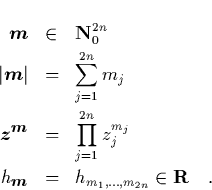
a fixed point in the origin. We can always write the Hamiltonian  as
a formal power series in the phase space coordinates
as
a formal power series in the phase space coordinates  ,
,  ,
,
 . With
 we have
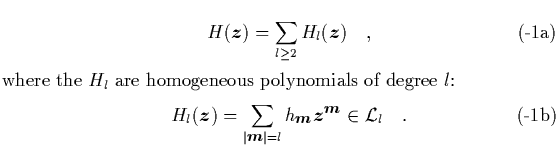
Here  is the
 -dimensional vector space of
homogeneous polynomials of degree
-dimensional vector space of
homogeneous polynomials of degree  in
in  variables, and we employ the
multiindex notation
variables, and we employ the
multiindex notation
Note that the dimension of grows rapidly with (e.g. for  we have
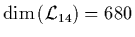 ), such that any manipulation of
 for larger values of
will have to be done by computer algebra rather than ``by hand''.
We denote the space of all formal power series beginning with degree 2 by
for larger values of
will have to be done by computer algebra rather than ``by hand''.
We denote the space of all formal power series beginning with degree 2 by
 .
.
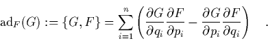
The Lie operator
 adjoint to a power series
  is the
Poisson bracket of
is the
Poisson bracket of  with some
  :
:
 |
(-1) |
is a linear operator on  for all .
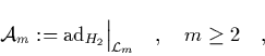
The Lie operator adjoint to the quadratic part of the
Hamiltonian and restricted to the subspace
for all .
The Lie operator adjoint to the quadratic part of the
Hamiltonian and restricted to the subspace  is of central
importance:
is of central
importance:
Note that  maps monomials of degree
  to
monomials of degree .
to
monomials of degree .
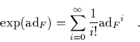
The Lie transformation associated with is the exponential
of
:
 |
(1) |
Lie transformations are an adequate tool for Hamiltonian normal form
theory because they are canonical [20].
Let be a Hamiltonian of type (1). is
in Birkhoff-Gustavson normal form up to order if
 |
(2) |
is in Birkhoff-Gustavson normal form if (6) holds
for all  .
This definition
is motivated by the fact that
.
This definition
is motivated by the fact that
 is an integral of motion if is in BGNF:
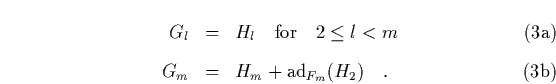
For any given Hamiltonian of type (1) we can proceed to
the BGNF of in the following way: With some  determine a
new Hamiltonian
determine a
new Hamiltonian
 by
by
 |
(3) |
More explicitely we have
where
 stands for terms of order
  and higher.
Collecting terms of equal order we get, using
and higher.
Collecting terms of equal order we get, using
 :
:
Assuming that is already in BGNF up to order  , equation
(8) allows several important conclusions: First of all,
according to (8a) the contributions of order less than
remain unchanged under the Lie transformation associated to
, equation
(8) allows several important conclusions: First of all,
according to (8a) the contributions of order less than
remain unchanged under the Lie transformation associated to  .
This shows that
the transformed Hamiltonian
.
This shows that
the transformed Hamiltonian  is
at least in normal form up to order , too.
Secondly, (8b) indicates how to obtain a Hamiltonian which
is in BGNF even up to order :
From (8b) we get
is
at least in normal form up to order , too.
Secondly, (8b) indicates how to obtain a Hamiltonian which
is in BGNF even up to order :
From (8b) we get
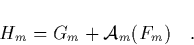 |
(3) |
This homological
equation [23] must be solved for and  under the
additional condition
under the
additional condition
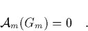 |
(4) |
In other words, must be in the kernel (or null space) of :
Thus we have the following iterative process for the normalization of :
For all  we first solve the homological equation for the
polynomials and and then obtain the remaining terms
we first solve the homological equation for the
polynomials and and then obtain the remaining terms  of the new Hamiltonian by evaluating (7). The
calculation of the
of the new Hamiltonian by evaluating (7). The
calculation of the  is a tedious but straight-forward task that can
be left to computer algebra. The non-trivial key point is solving the
homological equation.
is a tedious but straight-forward task that can
be left to computer algebra. The non-trivial key point is solving the
homological equation.
Let us assume that the vector space can be decomposed into the
direct sum of the kernel and range spaces of ,
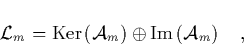 |
(5) |
with
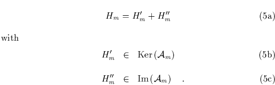
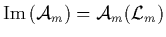 . Then
  can uniquely be split
into its kernel and range components
can uniquely be split
into its kernel and range components
Hence,
is uniquely determined by the kernel component of  :
:
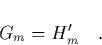 |
(5) |
Finally can be obtained by inverting
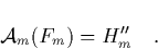 |
(6) |
Since there may be several preimages of  under
( is uniquely determined by (14) up to any
element of the null space of )
the normalization procedure is not unambiguous. However, we can always
achieve unambiguity by additionally requiring to lie in the range
space of .
under
( is uniquely determined by (14) up to any
element of the null space of )
the normalization procedure is not unambiguous. However, we can always
achieve unambiguity by additionally requiring to lie in the range
space of .
The key point of the above procedure is the splitting
(11). By means of the canonical transformation
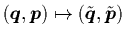 with
with
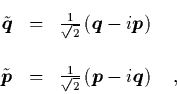 |
(7) |
Gustavson showed that for a Hamiltonian of type (1)
equation
(11) holds, since in the new coordinates
 the corresponding transformed operator
 is diagonal.
Since
yields the splitting (11),
does as well. This
proves the applicability of the BGNF theory to Hamiltonians of the
Gustavson type (1):
Every such Hamiltonian can, by means of a formal canonical
transformation, be transformed into the equivalent Hamiltonian
is diagonal.
Since
yields the splitting (11),
does as well. This
proves the applicability of the BGNF theory to Hamiltonians of the
Gustavson type (1):
Every such Hamiltonian can, by means of a formal canonical
transformation, be transformed into the equivalent Hamiltonian
![\begin{displaymath}
\quad
G = \Big[ \cdots \circ \exp\left(\mbox{\rm ad}_{F_4}...
...\circ \exp\left(\mbox{\rm ad}_{F_3}\right) \Big] \; (H) \quad,
\end{displaymath}](img68.png) |
(8) |
where and is in BGNF.
The term ``formal''
indicates that we do not yet consider
the convergence properties of the power series , and .
Next: The generalized normal form
Up: Normal forms
Previous: Normal forms
Contents
Martin_Engel
2000-05-25