Next: On the Interpretation as
Up: Quantum Phase Space Distribution
Previous: The HUSIMI Distribution Function
Contents
Since
 ,
for each
,
for each  ,
contains exactly the same information as
the HILBERT space vector
,
contains exactly the same information as
the HILBERT space vector
 it is possible to give a
complete formulation of quantum mechanics by means of phase space
distribution functions only, that is without referring to
quantum
state vectors or
wave functions. In such a framework describes the state of
the system at time
it is possible to give a
complete formulation of quantum mechanics by means of phase space
distribution functions only, that is without referring to
quantum
state vectors or
wave functions. In such a framework describes the state of
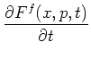
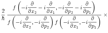
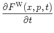
the system at time  , whereas the time evolution of is
determined by the equation of motion
, whereas the time evolution of is
determined by the equation of motion
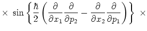
which takes the role normally occupied by the SCHRÖDINGER equation
in the conventional formulation of quantum
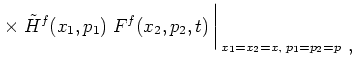
mechanics. Here,
 is the transform
of the Hamiltonian; it is obtained by first ordering the Hamiltonian
is the transform
of the Hamiltonian; it is obtained by first ordering the Hamiltonian
 according to the kernel function
 ,
as described in section A.1,
and then replacing the operators
,
as described in section A.1,
and then replacing the operators  ,
,  with
the scalars
with
the scalars  ,
,  .
COHEN was the first to formulate the equation of motion
(A.80) [Coh66];
a derivation starting from the VON NEUMANN equation
can
be found in [Lee95].
.
COHEN was the first to formulate the equation of motion
(A.80) [Coh66];
a derivation starting from the VON NEUMANN equation
can
be found in [Lee95].
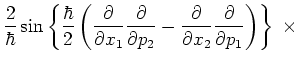
As an example, for the special case of the WIGNER distribution function
equation (A.80) becomes
Obviously, the equations of motion (A.80) and (A.81)
are quite awkward to work with. This is the most important reason why in
practical applications quantum mechanics hardly ever is discussed
with distribution functions completely replacing quantum
states and wave functions.
Rather, even when the final task is to obtain distribution functions,
typically the well-established version of quantum mechanics is used,
i.e. one starts
by solving -- numerically, if necessary -- the SCHRÖDINGER equation
and then inserts the solution
into equation
(A.13)
or (A.74), for instance,
in order to compute the desired .
But in addition to the computation of distribution functions, the equation
of motion for WIGNER's function is of importance for the
investigation of the
semiclassical approximation with
 .
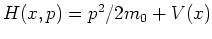
For Hamiltonians of the type
.
For Hamiltonians of the type
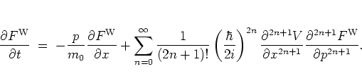
 equation (A.81) can be ordered with respect to powers of
 :
:
 |
(A.52) |
This equation was first
derived
by WIGNER in 1932 [Wig32].
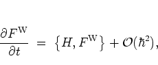
Using the POISSON bracket
 , it can be rewritten in the
form
, it can be rewritten in the
form
 |
(A.53) |
with
 as usual denoting terms that are at least
quadratic in and that give rise to the quantum mechanical
corrections to the classical phase space distribution function
as usual denoting terms that are at least
quadratic in and that give rise to the quantum mechanical
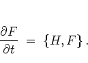
corrections to the classical phase space distribution function  as obtained from the classical LIOUVILLE equation
 |
(A.54) |
Therefore in the classical limit  the equation of motion
(A.83) for
the equation of motion
(A.83) for
 formally
becomes the LIOUVILLE equation (A.84);
this makes WIGNER's function a
useful tool for the investigation of the correspondence issue.
Furthermore, for potentials
formally
becomes the LIOUVILLE equation (A.84);
this makes WIGNER's function a
useful tool for the investigation of the correspondence issue.
Furthermore, for potentials  that do not contain powers of
exceeding 2, the dynamics of is completely
classical, since in this case the equations (A.83) and
(A.84) coincide.
But note that itself depends on , such that the
similarity
of these quantum mechanical and classical equations of motion
is formal in the first place, and
the details of obtaining equation (A.84) from
(A.83) in the classical limit are nontrivial in general.
that do not contain powers of
exceeding 2, the dynamics of is completely
classical, since in this case the equations (A.83) and
(A.84) coincide.
But note that itself depends on , such that the
similarity
of these quantum mechanical and classical equations of motion
is formal in the first place, and
the details of obtaining equation (A.84) from
(A.83) in the classical limit are nontrivial in general.
I
return
to equations (A.82) and
(A.83) in section A.5 when I discuss
the interpretation of as a (quasi-) probability
distribution function in quantum phase space.
Next: On the Interpretation as
Up: Quantum Phase Space Distribution
Previous: The HUSIMI Distribution Function
Contents
Martin Engel 2004-01-01