On the Interpretation as Probability
Densities

The motivation of the theory outlined in this appendix was to construct distribution functions which can play the same role in quantum mechanics as the conventional phase space probability densities do in classical mechanics (cf. pages ff). Therefore it now needs to be checked to what extent the functions $F^f(x,p,t)$ actually have the typical properties of probability densities.

A ``genuine'' phase space probability density $F(x,p,t)$ is characterized by the following properties:^A.12

1. Reality: $F(x,p,t)\in\mathbb{R}$ for all $x$, $p$ and $t$.
2. Positivity: $F(x,p,t)\geq 0$ for all $x$, $p$ and $t$.
3. By integration over $p$ and $x$, $F(x,p,t)$ must give the correct quantum mechanical marginal probability densities in position and momentum space, respectively:^A.13
   
   

The first two conditions are natural, since all probabilities that are to be computed using $F$ must be real-valued and non-negative as well. The third condition is necessary in order to obtain agreement with the usual Copenhagen interpretation of quantum mechanics, where the wave functions $\left< x \left\vert \psi(t) \right> \right.$ and $\left< p \left\vert \psi(t) \right> \right.$ take the role of probability amplitudes.

The properties (i)-(iii) are not automatically satisfied for all distribution functions $F^f$, but must be checked for each individual $f$. They are by no means necessary consequences of the definitions in sections A.1 and A.2. On the contrary, it can be shown that for nonzero $\hbar$ none of the known $F^f$ satisfies all three conditions. This may be interpreted as a consequence of HEISENBERG's uncertainty relation and was already observed by WIGNER in 1932 [Wig32]. This shortcoming of all distribution functions $F^f$ is the reason for using the prefix quasi in terms like quasiprobability density or quasiprobability distribution function.

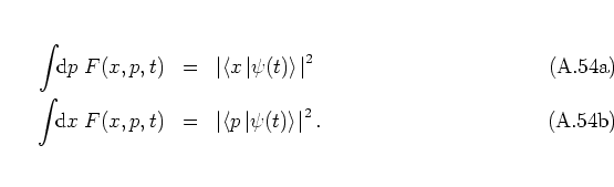
WIGNER's distribution function, for example, is real-valued and gives the correct marginal probability distributions for position and momentum, but it can take on negative values. In fact, it typically oscillates very rapidly and with large amplitude between positive and negative values under variation of $x$ or $p$. This behaviour of the WIGNER function is further discussed and demonstrated for some examples in section A.6.

For the antinormal-ordered and the HUSIMI distribution functions one has, using equations (A.51, A.74),

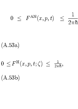
respectively. Both are real-valued and non-negative. They are even bounded and do not oscillate as rapidly as $F^{\rm W}$. But, on the other hand, they do not yield the correct probability densities for $x$ and $p$ by marginalization. Again I refer the reader to section A.6 for more details. Table A.1 gives an overview of the essential properties of the distribution functions defined in sections A.2 and A.3.

Table A.1: Properties of the WIGNER, standard-ordered, antistandard-ordered, normal-ordered, antinormal-ordered, HUSIMI and anti-HUSIMI distribution functions.

distribution function		real-valued	non-negative	correct marginal
					distributions
$F^{\rm W}$		$(x,p,t)$	yes	no	yes
$F^{\rm S}$		$(x,p,t)$	no	no	yes
$F^{\rm AS}$		$(x,p,t)$	no	no	yes
$F^{\rm N}$		$(x,p,t)$	yes	no	no
$F^{\rm AN}$		$(x,p,t)$	yes	yes	no
$F^{\rm H}$		$(x,p,t;\zeta)$	yes	yes	no
$F^{\rm AH}$		$(x,p,t;\zeta)$	yes	no	no

It is important to keep in mind that despite the different properties of the distribution functions, they are all equivalent in the sense that all of them contain exactly the same information about the state of the system. This can be exploited by choosing that type of distribution function $F^f$ (respectively by choosing that kernel function $f$) that is most suited to study the particular problem in question.

For the purpose of comparing the classical and quantum mechanical equations of motion of a given system, one usually uses WIGNER's function (cf. equation (A.82); see [Bun95] for details). $F^{\rm W}$ is also especially well suited for the discussion of scattering systems, because in such systems, for large energies, the classical limiting case often is a good approximation to the exact quantum system already; equation (A.82) can then be used to determine the quantum correction terms in a systematic way. On the other hand, if the quantum and classical phase space (quasi-) probability densities themselves are in the focus of attention, then most frequently the HUSIMI distribution function $F^{\rm H}$ or the coherent state representation $F^{\rm AN}$ are employed. In section A.6 I discuss some of the advantages of this choice by considering two familiar quantum states as examples.

Footnotes

... properties:^A.12

There are further, more technical conditions that are to be satisfied by a probability density [Lee95]; these additional properties are not needed for the present discussion.

... respectively:^A.13

Equations (A.85a, A.85b) are just two specific examples for the marginalization of a distribution function. Generally speaking, a marginalization of a distribution function $F$ is a line integral over $F$ in phase space. In equations (A.85a, A.85b), the line integrals are taken along the $p$ and $x$ axes of phase space, respectively. More on marginalizations of distribution functions may be found in [MMT97].