The first point to note when it comes to the practical application of
phase space distribution functions is that their numerical computation for
a given quantum state
![]() does not cost as much effort as it
might seem at first sight of equations like (A.13).
For example, the WIGNER function can be written as
does not cost as much effort as it
might seem at first sight of equations like (A.13).
For example, the WIGNER function can be written as
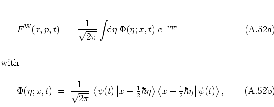
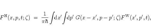
and for the HUSIMI distribution one has
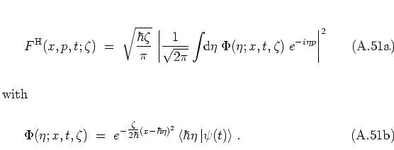
These expressions show that both
![]() and
and ![]() can be computed efficiently
from
can be computed efficiently
from
![]() by FOURIER transformation,
and the same is true for other
by FOURIER transformation,
and the same is true for other
![]() as well.
Typically the method of fast FOURIER transformation (FFT)
[CT65,EMR93] is employed here which
drastically reduces the numerical effort, as compared with conventional
methods of computation.A.14
as well.
Typically the method of fast FOURIER transformation (FFT)
[CT65,EMR93] is employed here which
drastically reduces the numerical effort, as compared with conventional
methods of computation.A.14
In the literature, initially mainly the WIGNER function has been used. But in the last years the situation has changed in favour of the HUSIMI function which is in widespread use by now. In the following I want to motivate this transition with two arguments, the first being analytical while the second is a numerical example of a typical application.
In the context of HUSIMI functions, equation (A.31) can be
written as
The numerical example below shows that the rapid oscillations of the
WIGNER function have no obvious counterpart in the classical phase
portrait, whereas the phase space patterns of the HUSIMI function
follow the classical structures much more closely. In this sense the
smoother HUSIMI function can be interpreted as a (quasi-) probability
density in a much more intuitive way than the WIGNER function.
This property makes ![]() the first choice distribution function
for the purpose of visualization of quantum nonlinear dynamical systems,
especially when the classical dynamics is chaotic.
the first choice distribution function
for the purpose of visualization of quantum nonlinear dynamical systems,
especially when the classical dynamics is chaotic.
A
parallel
argument explains why the normal-ordered distribution function
is utilized rarely and why the anti-HUSIMI distribution function is
not used at all for
creating an intuitive picture of a quantum state.
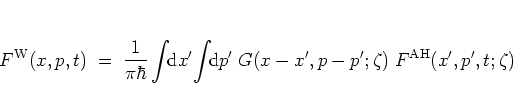
Similar
to equation
(A.89) one has
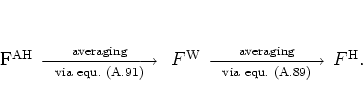
Finally there exists a strong argument in favour of the HUSIMI distribution from the experimenters' point of view: TAKAHASHI and
SAITÔ argue that ![]() is much better suited to any
experimental setup than
is much better suited to any
experimental setup than ![]() since the averaging in equation
(A.89) acts in a similar way as the coarse graining effect that
is inherent to all experimental measurement processes
[TS85].
In a particular experimental setup, on the other hand, the WIGNER function still has the striking advantage that it can be measured
directly
at each point of phase space,
without the need for any further complex
computation: in [MCK93] it is shown that, after some
algebra,
since the averaging in equation
(A.89) acts in a similar way as the coarse graining effect that
is inherent to all experimental measurement processes
[TS85].
In a particular experimental setup, on the other hand, the WIGNER function still has the striking advantage that it can be measured
directly
at each point of phase space,
without the need for any further complex
computation: in [MCK93] it is shown that, after some
algebra, ![]() can be written as
can be written as
At this point one is now in the position to
further
interpret the additional
``squeezing''
parameter ![]() of the (anti-) HUSIMI distribution. Equations
(A.89, A.91)
show that
of the (anti-) HUSIMI distribution. Equations
(A.89, A.91)
show that ![]() controls the way in
which the averaging discussed above is performed, namely by specifying
the width of the Gaussian (A.90)
in
controls the way in
which the averaging discussed above is performed, namely by specifying
the width of the Gaussian (A.90)
in ![]() - and
- and ![]() -direction.
The effective area over which is averaged is an
ellipse
with widths
-direction.
The effective area over which is averaged is an
ellipse
with widths
![]() and
and
![]() in
in ![]() - and
- and ![]() -direction,
respectively
-- compare these values
with the uncertainties (A.64) of general squeezed states.
Therefore, larger values of
-direction,
respectively
-- compare these values
with the uncertainties (A.64) of general squeezed states.
Therefore, larger values of ![]() yield an averaging area that is
squeezed
in the direction of
yield an averaging area that is
squeezed
in the direction of ![]() and
broadened
in the direction of
and
broadened
in the direction of ![]() .
The particular choice
.
The particular choice ![]() , which is used
in many applications
and corresponds to the coherent state representation (A.51),
accordingly specifies a circular averaging area.
, which is used
in many applications
and corresponds to the coherent state representation (A.51),
accordingly specifies a circular averaging area.
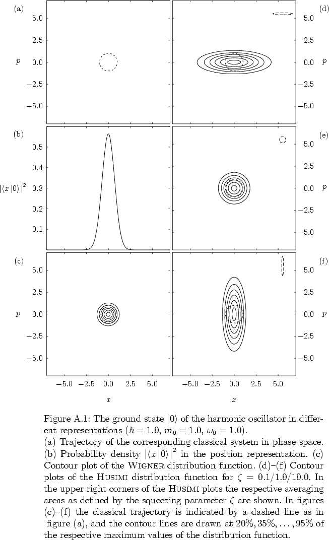
In order to exemplify the above statements, in figures
A.1-A.3
I compare the most important ways to graphically
represent quantum states. The states used for this demonstration are
the familiar ground state
![]() of the harmonic oscillator and its
tenth eigenstate
of the harmonic oscillator and its
tenth eigenstate
![]() .
.
Figure A.1a shows a classical phase space trajectory of
the harmonic oscillator at the energy
![]() .
The corresponding quantum mechanical wave function in the position
representation (figure A.1b) bears no obvious resemblance
to the classical trajectory and is therefore of little use for the
purpose of comparing the classical and quantum states. For this purpose,
figure A.1c is much better suited: the contour plot of the
WIGNER function of
.
The corresponding quantum mechanical wave function in the position
representation (figure A.1b) bears no obvious resemblance
to the classical trajectory and is therefore of little use for the
purpose of comparing the classical and quantum states. For this purpose,
figure A.1c is much better suited: the contour plot of the
WIGNER function of
![]() that is shown here is essentially a
bell-shaped function that is peaked at the origin of phase space -- near
the classical trajectory. The contour plots of the HUSIMI distributions
for different values of
that is shown here is essentially a
bell-shaped function that is peaked at the origin of phase space -- near
the classical trajectory. The contour plots of the HUSIMI distributions
for different values of ![]() in
figures A.1d-A.1f
are not
much more informative; all of them show bell-shaped curves centered about
the origin. Note that the HUSIMI function for
in
figures A.1d-A.1f
are not
much more informative; all of them show bell-shaped curves centered about
the origin. Note that the HUSIMI function for ![]() is the one that
is closest to the classical trajectory, since for
is the one that
is closest to the classical trajectory, since for ![]() one
obtains distributions that do not reproduce the classical rotational
symmetry of the trajectory.
one
obtains distributions that do not reproduce the classical rotational
symmetry of the trajectory.
While the advantages of the HUSIMI distribution are not obvious with
respect to the simple ground state
![]() they become clearly visible
when more
complex
states are considered.
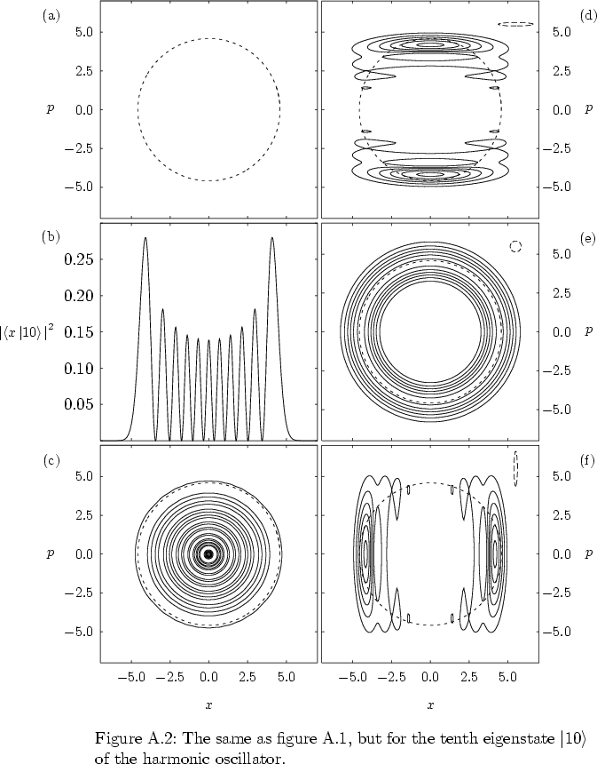
Figure A.2 shows the same kind of plots as figure
A.1 but now for the state
they become clearly visible
when more
complex
states are considered.
Figure A.2 shows the same kind of plots as figure
A.1 but now for the state
![]() .
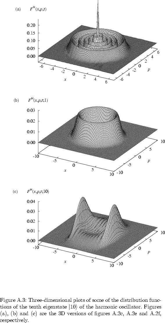
The highly oscillatory character of the WIGNER function is illustrated
in the contour plot A.2c and in its three-dimensional
counterpart in figure A.3a. These plots do not show
much similarity to the corresponding classical path in figure
A.2a.
.
The highly oscillatory character of the WIGNER function is illustrated
in the contour plot A.2c and in its three-dimensional
counterpart in figure A.3a. These plots do not show
much similarity to the corresponding classical path in figure
A.2a.
Only when turning to the HUSIMI distribution in figures
A.2d-A.2f
-- and in figures
A.3b, A.3c
with the 3D versions
--
(some aspects of) the classical trajectory can be
identified in quantum phase space. This is best achieved for ![]() :
:
![]() essentially is a circular ridge which takes on its
maximum value at the points of the classical trajectory. For
essentially is a circular ridge which takes on its
maximum value at the points of the classical trajectory. For ![]() and
and ![]() rotational invariance is lost and two characteristic peaks
emerge with no obvious counterpart in the classical picture. But
even in these cases the location of the classical path can clearly be
identified.
rotational invariance is lost and two characteristic peaks
emerge with no obvious counterpart in the classical picture. But
even in these cases the location of the classical path can clearly be
identified.