The characteristic property of an integral of motion is its constancy
along trajectories in phase space. As mentioned earlier, one cannot
expect this behaviour for a formal integral of a nonintegrable system like
the magnetic bottle discussed here. But in line with reference
[28] (and many others) we still expect convergence
of
![]() in regular regions of phase space.
in regular regions of phase space.
Let us define the quasi-integral
![]() of order
of order ![]() as that
approximation to
as that
approximation to
![]() that contains only monomials of degree
that contains only monomials of degree ![]() and less:
and less:
The above analysis is local in the sense that one has to specify a
single point
![]() for which
for which
![]() ist evaluated. We
now turn
to a kind of global analysis and show how to obtain a qualitative
picture of the convergence properties of
ist evaluated. We
now turn
to a kind of global analysis and show how to obtain a qualitative
picture of the convergence properties of
![]() in a larger region
of phase space.
in a larger region
of phase space.
In order to have a (though somewhat strong)
criterion for convergence we
say that
![]() is convergent at
is convergent at
![]() if
if
The next step is to define a convergence function
![]() by setting
by setting
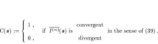 |
(30) |
In figure 5 we present a convergence plot for the
magnetic bottle (33) at the energy ![]() . This picture
should be compared with figure 3b. On a
. This picture
should be compared with figure 3b. On a
![]() grid we have marked with black all points where
grid we have marked with black all points where
![]() indicates
convergence of the quasi-integral.
It is interesting to see that although the condition
(39) is quite strong there are large convergent regions
in
indicates
convergence of the quasi-integral.
It is interesting to see that although the condition
(39) is quite strong there are large convergent regions
in ![]() . Many of the details of the Poincaré plot
3b show up in the convergence plot as well. As expected,
convergence is most frequent in the centre of the picture. Furthermore,
the hyperbolic periodic points of the two dominant Birkhoff chains
(of period four and six, respectively) in figure 3b are
clearly represented in figure
5 by clouds of black marks. This is
surprising, because in the neighbourhoods of these hyperbolic points
one would expect distinct divergent behaviour, caused by the chaotic
dynamics in a heteroclinic tangle scenario.
. Many of the details of the Poincaré plot
3b show up in the convergence plot as well. As expected,
convergence is most frequent in the centre of the picture. Furthermore,
the hyperbolic periodic points of the two dominant Birkhoff chains
(of period four and six, respectively) in figure 3b are
clearly represented in figure
5 by clouds of black marks. This is
surprising, because in the neighbourhoods of these hyperbolic points
one would expect distinct divergent behaviour, caused by the chaotic
dynamics in a heteroclinic tangle scenario.
As an aside we
remark that the convergence of the quasi-integral
for the magnetic bottle considered here is worse than the convergence for
the Hénon-Heiles system discussed in [28]. This seems
to be due to the fact that for the latter system the accessible region of
phase space is bounded, whereas for the magnetic bottle the dynamical
region extends infinitely along the ![]() -axis.
-axis.
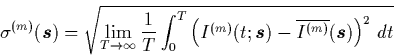
In order to get refined information about the convergence properties of
the
![]() as a function of
as a function of ![]() we now modify the rule for
marking points in the convergence plot.
As a measure for the deviation of
we now modify the rule for
marking points in the convergence plot.
As a measure for the deviation of
![]() from its mean value
we calculate the standard deviation
from its mean value
we calculate the standard deviation
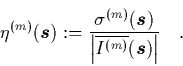
Again we can mark the points of the surface of section of the magnetic
bottle, this time according to the value of
![]() . The result
can be seen in figure 7 which is to be compared
with the Poincaré plots of figure 3. The dark regions
correspond to larger values of
. The result
can be seen in figure 7 which is to be compared
with the Poincaré plots of figure 3. The dark regions
correspond to larger values of
![]() , thus indicating -- cum grano salis -- convergence, while points in the light grey or white
areas have small
, thus indicating -- cum grano salis -- convergence, while points in the light grey or white
areas have small
![]() , which means that
, which means that
![]() increases quite from the beginning.
The Poincaré plot 3a at a very low energy shows
regular motion, and figure 7a accordingly indicates
convergence in large regions of
increases quite from the beginning.
The Poincaré plot 3a at a very low energy shows
regular motion, and figure 7a accordingly indicates
convergence in large regions of ![]() .
The light grey spots in the centre of the figure must not be mistaken as
indicating divergent behaviour. On the contrary, convergence is excellent
around the origin, such that very small values of
.
The light grey spots in the centre of the figure must not be mistaken as
indicating divergent behaviour. On the contrary, convergence is excellent
around the origin, such that very small values of
![]() are being compared, and values of
are being compared, and values of
![]() larger than two are due
to the limited accuracy of the numerical calculation and round-off.
Convergence deteriorates with
increasing
larger than two are due
to the limited accuracy of the numerical calculation and round-off.
Convergence deteriorates with
increasing ![]() (und thus increasing chaoticity) as the comparison of
figures 3b,c and 7b,c shows.
Especially figure 7b reproduces the content of the
Kaluza-Robnik-type picture 5 very well and even
adds on much more information about the convergent regions.
We conclude that the
(und thus increasing chaoticity) as the comparison of
figures 3b,c and 7b,c shows.
Especially figure 7b reproduces the content of the
Kaluza-Robnik-type picture 5 very well and even
adds on much more information about the convergent regions.
We conclude that the
![]() -plots are considerably better
suited than the
-plots are considerably better
suited than the
![]() -plots for the analysis of the convergence
properties of the quasi-integral.
-plots for the analysis of the convergence
properties of the quasi-integral.
It
is important to keep in mind that we are using quite a special
definition of ``convergence'' here. While this is useful for the present
discussion, comparison with rigorous theoretical results about the
divergence mechanism [31,32]
is delicate. Generally, (pseudo-) convergence (in the usual sense) is
expected within a disc, which is compatible with figures
5 and 7a.
But figure 7b seems to indicate that convergence has spread
into the region between the island chains of period four and six, at
variance to the theoretical prediction. The reason being that
![]() or 4 reflects only the behaviour for the first few orders
or 4 reflects only the behaviour for the first few orders
![]() and is no direct indicator for true convergence. So the values of
and is no direct indicator for true convergence. So the values of
![]() can be taken only as a vague phenomenological hint
towards true convergence or divergence.
can be taken only as a vague phenomenological hint
towards true convergence or divergence.
Figure 7b already reproduces reasonably well the features of
the corresponding Poincaré plot, but only in regions not too far away
from the origin. In an attempt to enlarge the region that is accessible
for the analysis we make the following exponential ansatz for the
normalized standard deviations as functions of ![]() :
:
It is one of the advantages of the
![]() -method that one
obtains a continuous spectrum of values of
-method that one
obtains a continuous spectrum of values of
![]() , as opposed
to the discrete spectra of
, as opposed
to the discrete spectra of
![]() and
and
![]() .
This becomes apparent in figure 9 where we show again
.
This becomes apparent in figure 9 where we show again
![]() , now shaded according to
, now shaded according to
![]() .
The lighter the grey, the larger
.
The lighter the grey, the larger
![]() and thus the faster
the divergence of the quasi-integral. The central portion of the picture
is similar to the one of figure 7b, but now the outer
regions show some structure, too. Comparing with the corresponding
Poincaré plot (figure 3b) one sees that the
and thus the faster
the divergence of the quasi-integral. The central portion of the picture
is similar to the one of figure 7b, but now the outer
regions show some structure, too. Comparing with the corresponding
Poincaré plot (figure 3b) one sees that the
![]() -plot clearly marks the third and fourth largest
Birkhoff chains as well. And even more structure can be detected by
more careful analysis of the picture. So the ansatz
(42) seems to be justified.
-plot clearly marks the third and fourth largest
Birkhoff chains as well. And even more structure can be detected by
more careful analysis of the picture. So the ansatz
(42) seems to be justified.