We consider a ``magnetic bottle'' which is made up of a homogeneous
magnetic (dipole) field with a superimposed octupole contribution. In
cylindrical coordinates we have:
We
restrict ourselves to the case
![]() , such that a particle in the bottle does not encircle the
, such that a particle in the bottle does not encircle the
![]() -axis but continually passes through it.
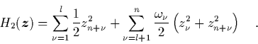
After suitable scaling we arrive (for
-axis but continually passes through it.
After suitable scaling we arrive (for ![]() ) at the Hamiltonian
) at the Hamiltonian
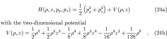
![]() describes a system with two degrees of freedom, one of which (
describes a system with two degrees of freedom, one of which (![]() )
corresponds, in lowest order approximation, to a harmonically bound motion
while the dynamics along the
)
corresponds, in lowest order approximation, to a harmonically bound motion
while the dynamics along the ![]() -axis is free in the same
approximation.
Note that this Hamiltonian cannot be dealt with by
the BGNF theory.
-axis is free in the same
approximation.
Note that this Hamiltonian cannot be dealt with by
the BGNF theory.
In what follows, we do not restrict ![]() to positive values but allow
for negative values as well. This makes it possible to treat
to positive values but allow
for negative values as well. This makes it possible to treat ![]() and
and
![]() simply as cartesian coordinates in two dimensions.
An example for the dynamics of our model system, obtained by numerical
integration, is shown in figure 2.
Similarly, we have numerically calculated Poincaré plots for several
energies
simply as cartesian coordinates in two dimensions.
An example for the dynamics of our model system, obtained by numerical
integration, is shown in figure 2.
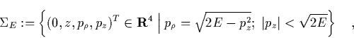
Similarly, we have numerically calculated Poincaré plots for several
energies ![]() . To this end we have defined Poincaré surfaces of
section
. To this end we have defined Poincaré surfaces of
section ![]() by setting
by setting ![]() ,
,
It is important to realize that for this system a global second integral of motion (the first being the Hamiltonian itself) cannot exist, because the existence of such an integral would render the system integrable. This would be incompatible with the non-integrability demonstrated by the Poincaré plots. Still, the preceding section shows how to construct a formal invariant. The resolution of this ostensible contradiction is that one expects the formal integral to approximate the local exact integrals of motion in the regular regime (where the KAM tori dominate) whereas in the stochastic regions the formal integral is expected to diverge. See [28] for a discussion of these convergence properties.
Rather than discussing just the Hamiltonian (33) we will
study the normalization process for the more general class of
magnetic bottle Hamiltonians
which are defined by their quadratic contribution:
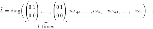
Transformation of the corresponding Hamiltonian matrix
![]() into Jordan normal form yields
into Jordan normal form yields
The stage is set for application of the normalization process as
described in section 2.
In the appendix we explain in some detail how
the effort needed to normalize magnetic bottle Hamiltonians can be
reduced considerably.
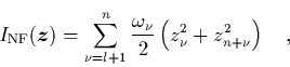
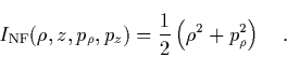
As the result of these considerations we have obtained the formal integral
of the magnetic bottle (33) up to and including the
14th order. The first few terms are
It is important to note the difference between the representations (37) and (38) of the integral of motion. The first formula applies if the Hamiltonian is already in generalized normal form, while the second holds for the non-normalized Hamiltonian (33) in the original coordinates and is obtained from (37) by inverting the normalizing Lie transformations.
To our knowledge, there is only one other example in the literature where
normalization for a full Hamiltonian has been carried out up to
such a high order [28,29]. (Discrete mappings,
on the other hand, have been normalized up to order 100 and beyond; cf. [30].)
One has to realize, though, that the
Hénon-Heiles Hamiltonian considered in
[28,29]
is of the Gustavson
type (1), thus rendering ![]() diagonal.
As explained in the appendix, for magnetic bottle
Hamiltonians
diagonal.
As explained in the appendix, for magnetic bottle
Hamiltonians ![]() is not diagonal, which makes the determination
of the splitting (12) and the inversion of
(14) a much more difficult task.
is not diagonal, which makes the determination
of the splitting (12) and the inversion of
(14) a much more difficult task.
![\begin{displaymath}
\quad
{\mbox{\protect\boldmath$B$}}(\rho,z) := B_0{\mbox{\...
...2}\rho^2\right){\mbox{\protect\boldmath$e$}}_z \right]
\quad.
\end{displaymath}](img176.png)