


Next: Singular Value Decomposition as
Up: Singular System Analysis
Previous: Singular System Analysis
Contents
As a first step we choose some  . We want to embed
  in
in
 . In general
  will be unknown so that it is not obvious how
to meet Takens' condition
will be unknown so that it is not obvious how
to meet Takens' condition  . But if we choose large enough to
ensure that
. But if we choose large enough to
ensure that  then we can embed in ,
according to Takens' theorem 2, because it is a well known fact that
every Euclidean space
then we can embed in ,
according to Takens' theorem 2, because it is a well known fact that
every Euclidean space
 can again be embedded in any
higher-dimensional Euclidean space without any problems.
So we start by making an ansatz for and our concern for the
next few paragraphs will be to find a more appropriate
can again be embedded in any
higher-dimensional Euclidean space without any problems.
So we start by making an ansatz for and our concern for the
next few paragraphs will be to find a more appropriate  such that
  is a space containing Takens' embedding space.
Thus
is a space containing Takens' embedding space.
Thus  will be a better embedding dimension than the we started
with, since it gives a lower-dimensional embedding space.
We want to use the method of delays to construct vectors in
from the
will be a better embedding dimension than the we started
with, since it gives a lower-dimensional embedding space.
We want to use the method of delays to construct vectors in
from the  of the time series. Doing this one realizes that there is
even one more quantity which is not yet specified: One could, for example,
take the series of -vectors
of the time series. Doing this one realizes that there is
even one more quantity which is not yet specified: One could, for example,
take the series of -vectors
 |
(27) |
which we are obviously allowed to use in accordance with Takens'
statements. So we also have to choose the ``lag time''
 , where
  . We will see in section 3.4.2
that we do not have to spend much effort on choosing
. We will see in section 3.4.2
that we do not have to spend much effort on choosing  :
when we use the singular systems technique the
influence of the lag time becomes insignificant, hence we will choose it
from now on to equal
:
when we use the singular systems technique the
influence of the lag time becomes insignificant, hence we will choose it
from now on to equal  (i.e.
(i.e.  ).
Consider a sequence of
).
Consider a sequence of  vectors
 ,
,
 (i.e. we take a time series containing
  data
points)12.
There seems to be no analytical way to compute the proper (i.e.
minimal) embedding
dimension from the time series. However, it is possible to determine a
reasonable estimate for it: For some given the -vectors
data
points)12.
There seems to be no analytical way to compute the proper (i.e.
minimal) embedding
dimension from the time series. However, it is possible to determine a
reasonable estimate for it: For some given the -vectors  usually do not explore the whole space . Rather than that they
are restricted to some subspace
usually do not explore the whole space . Rather than that they
are restricted to some subspace  of ; T contains the
embedded manifold which contains the picture of the attractor:
of ; T contains the
embedded manifold which contains the picture of the attractor:
 |
(28) |
When we assume that
the really visit the whole attractor in the
embedding space (more or less) uniformly and we bear in mind that
usually is much larger than then
 is a sensible
upper bound for the minimal embedding dimension. In order to determine we
compute the maximum number of linearly independent vectors that can be
constructed as linear combinations of the . To do this, we define the
is a sensible
upper bound for the minimal embedding dimension. In order to determine we
compute the maximum number of linearly independent vectors that can be
constructed as linear combinations of the . To do this, we define the
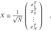
 -trajectory matrix
  :
:
 |
(29) |
which is built out of all vectors we want to use to reconstruct the
attractor.
Notice that when operating with  on some -vector we get an
-vector:
on some -vector we get an
-vector:
 |
(30) |
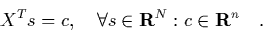
Since we are interested in linearly independent -vectors, we choose a
set of vectors
 such that the -vectors
 |
(31) |
are orthonormal. We introduce some real constants
 into this equation, in order to normalize the
  :
:
 |
(32) |
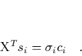
The important point about this equation is that, after transposing, it
can be rewritten as
 |
(33) |
i.e. as a linear combination of the reconstructed trajectory vectors.
This tells us, when we keep in mind the definition of , that we can
get linearly independent vectors  , using eq. (34); so we
have vectors
, using eq. (34); so we
have vectors  and numbers
 , too. The
 are elements of an orthonormal basis
 of .
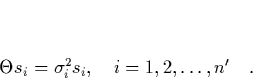
Thus we are left to determine as the number of those
of .
Thus we are left to determine as the number of those  which
are non-zero.
Define the structure matrix
which
are non-zero.
Define the structure matrix
 ; then it follows
from eq. (34) that the
; then it follows
from eq. (34) that the  are the eigenvalues of this
matrix:
are the eigenvalues of this
matrix:
 |
(34) |
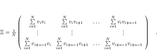
We could determine as the number of the non-zero eigenvalues of
 . But is a huge
  -matrix, and singular, and its
diagonalization is in practice impossible. Instead, we notice that the
covariance matrix
-matrix, and singular, and its
diagonalization is in practice impossible. Instead, we notice that the
covariance matrix
 has the same non-zero
eigenvalues as , and
has the same non-zero
eigenvalues as , and  is much easier to diagonalize, because it is only an
  -matrix. So
all one has to do in order to calculate which, cum grano salis,
estimates the minimal embedding dimension
-matrix. So
all one has to do in order to calculate which, cum grano salis,
estimates the minimal embedding dimension  , is to determine the
number of the non-zero eigenvalues of
, is to determine the
number of the non-zero eigenvalues of
 |
(35) |
Now we know that the trajectory is confined to an -dimensional
subspace of , and we can use as the embedding
space.
However, this treatment only makes sense in the case that we have noise-
free data.
Footnotes
- ...
points)12
-
We will generally assume
 , which is obviously true in most
cases.
, which is obviously true in most
cases.
Next: Singular Value Decomposition as
Up: Singular System Analysis
Previous: Singular System Analysis
Contents
Martin_Engel
2000-05-25