Next: Theoretical Foundation - Takens'
Up: Geometry from an Ideal
Previous: Geometry from an Ideal
Contents
The first group to propose a solution for the problem of
extracting geometric information from time series was Packard et
al. [3]. The basic idea of their approach is that the state
of an  -dimensional dynamical system can be uniquely
characterized by independent quantities. One such set of independent
quantities are, of course, the phase space coordinates (more exact: the
coordinates in some -dimensional basis which spans
-dimensional dynamical system can be uniquely
characterized by independent quantities. One such set of independent
quantities are, of course, the phase space coordinates (more exact: the
coordinates in some -dimensional basis which spans  )
)
 |
(8) |
but these are not available, since the only data one has is the
one-dimensional time series. Based on the conjecture that
any -tupel of numbers should give equivalent results
(in the sense that, if one reconstructs several phase portraits in
accordance with this idea, then for any two of these phase portraits
there should be a diffeomorphism which maps one onto the other)
Packard et al. proposed two
different possibilities to construct -vectors which in some sense
contain the same information as the original state vectors in eq.
(8):
One can work with the method of delays which simply takes
consecutive elements of the time series directly as coordinates in
phase space:
 |
(9) |
For example when analyzing a dynamical system it is often convenient just
to take one coordinate of phase space as the observable  :
:
 |
(10) |
The other possibility suggested by Packard et al. is to use the time
series to construct time
derivatives of the measured observable2 and use the vectors
 |
(11) |
In this way the one-dimensional time series is used to build a sequence of
-dimensional vectors which form a trajectory in some -dimensional
space.
Numerical experiments done by Packard et al. show that this procedure
gives reasonable results: the phase-space pictures one gets seem closely
related to the corresponding pictures of the original dynamical system.
In particular, topological properties and the geometrical form of the
attractor seem to be conserved under this procedure.
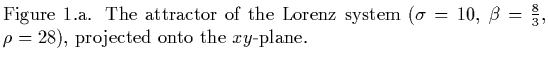
As an illustration of this method of phase space reconstruction, we
present a result of Broomhead and King [7]: They considered the
Lorenz system:
(with the parameter values  ,
,
 ,
,  ).
First they integrated this set of ordinary differential equations to get
the ``complete solution''; the projection of this solution onto the
).
First they integrated this set of ordinary differential equations to get
the ``complete solution''; the projection of this solution onto the
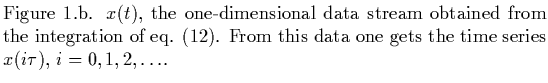
 -plane is shown in Fig. 1.a. They chose the
 -coordinate to be their ``observable'' and thus got the
one-dimensional data stream as shown in Fig. 1.b. Then,
after choosing some delay time
-coordinate to be their ``observable'' and thus got the
one-dimensional data stream as shown in Fig. 1.b. Then,
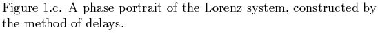
after choosing some delay time  , they obtained a discrete time
series from the data stream and used this time series to construct a
phase portrait, using the method of delays: See Fig. 1.c.
Comparison of the original Lorenz attractor
(Fig. 1.a) and the reconstructed one justifies Packard's
approach: Although the pictures are not exactly the same and although
Fig. 1.a is much coarser than Fig. 1.c, both
of them seem to show an object with the same geometry.
A shortcoming of Packard's method is that it does not give a general
strategy how to choose . If one knows that the dynamical system is
evolving in
, they obtained a discrete time
series from the data stream and used this time series to construct a
phase portrait, using the method of delays: See Fig. 1.c.
Comparison of the original Lorenz attractor
(Fig. 1.a) and the reconstructed one justifies Packard's
approach: Although the pictures are not exactly the same and although
Fig. 1.a is much coarser than Fig. 1.c, both
of them seem to show an object with the same geometry.
A shortcoming of Packard's method is that it does not give a general
strategy how to choose . If one knows that the dynamical system is
evolving in  -dimensional phase space then one can use the idea
mentioned above and take
-dimensional phase space then one can use the idea
mentioned above and take  . But if one is analyzing a system about the
dimensionality of which nothing is known a priori then how to proceed?
This problem will be addressed in section 3.
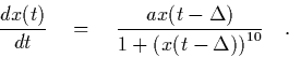
It is also not quite clear what should be when we try to reconstruct
phase portrait of a system with infinitely many degrees of freedom, such
as the Mackey-Glass equation ([5,12] and [14],
chapter 5.3):
. But if one is analyzing a system about the
dimensionality of which nothing is known a priori then how to proceed?
This problem will be addressed in section 3.
It is also not quite clear what should be when we try to reconstruct
phase portrait of a system with infinitely many degrees of freedom, such
as the Mackey-Glass equation ([5,12] and [14],
chapter 5.3):
 |
(13) |
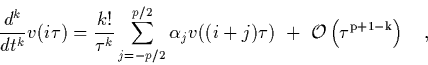
Footnotes
- ... observable2
-
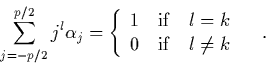
One can compute an approximation to the derivatives from the time
series for example by using the formula
where the  are determined by
This formula results from differentiating the interpolating polynomial.
See [10], §§ 27 and 28, for details of this method of
numerical differentiation.
See [11], chapter 3.4, for a more sophisticated extrapolation
method.
Next: Theoretical Foundation - Takens'
Up: Geometry from an Ideal
Previous: Geometry from an Ideal
Contents
Martin_Engel
2000-05-25