Next: Analysis of Real-World Data
Up: Geometry from an Ideal
Previous: The Principle of Reconstruction
Contents
Apparently without knowing about the work of Packard et al.,
Floris Takens gave their approach a safe theoretical foundation
[4]. Although different in details such as the dimension of
the reconstructed phase space, the spirit of his work is much the same.
Perhaps inspired by Whitney's embedding theorem, which states that every
 -dimensional manifold (of class
  ,
,
 )
can be embedded (via a diffeomorphism) in
)
can be embedded (via a diffeomorphism) in
 -dimensional Euclidean
space3, Takens
proposed to embed the attractor-manifold
-dimensional Euclidean
space3, Takens
proposed to embed the attractor-manifold  (i.e. the -dimensional
manifold which contains the attractor
(i.e. the -dimensional
manifold which contains the attractor  ) in
) in
 .
A smooth map
.
A smooth map
 , where
  and
and  are smooth
manifolds, embeds in (``is an embedding'') if
are smooth
manifolds, embeds in (``is an embedding'') if  is a
diffeomorphism from to a smooth submanifold of . is
called the embedding space; the embedding dimension is
is a
diffeomorphism from to a smooth submanifold of . is
called the embedding space; the embedding dimension is  .
Notice that, in general, we have
.
Notice that, in general, we have
 4. The notion of embeddings comes into the game
here, since one can think of
4. The notion of embeddings comes into the game
here, since one can think of  as being the realization of
as a submanifold of : The topological structures of and
as being the realization of
as a submanifold of : The topological structures of and
 are diffeomorphically equivalent. See Fig. 2.
This means that if we can find, using Takens' method, the embedding
which maps from to
then we can analyze the structure
of the trajectory of the dynamical system in
and then
easily from this infer properties of the actual trajectory on the
attractor in . Consider, for example, the dynamical system in eq.
(1); the embedding would tell us that there is a
dynamical system
are diffeomorphically equivalent. See Fig. 2.
This means that if we can find, using Takens' method, the embedding
which maps from to
then we can analyze the structure
of the trajectory of the dynamical system in
and then
easily from this infer properties of the actual trajectory on the
attractor in . Consider, for example, the dynamical system in eq.
(1); the embedding would tell us that there is a
dynamical system
and it follows already from ``topological equivalence'' (for which we even
only need to have a homeomorphism instead of a diffeomorphism)
that [7]:
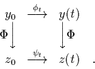
The dynamical systems of eqs. (1) and (14) are said to
have the same qualitative dynamics. This situation is represented
pictorially in Fig. 3.
It is especially nice to have the embedding if one wants to
characterize the dynamics of the system quantitatively: In this case
the dimensions (Hausdorff, topological, correlation, ...) of the attractor
in and in
are the same [8].
Takens stated the following theorem (theorem 2 in
[4]):
Given a compact -dimensional manifold , with  a
a
 -vector field (
 being the generating vector field of the
flow
being the generating vector field of the
flow  )
and
)
and
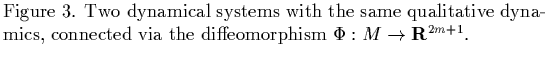
 a -function, define
Then, generically,  is an embedding.
Here, the term ``generically'' is of central importance:
The proof of this theorem is based on the idea that, if is
an embedding, then for all points
is an embedding.
Here, the term ``generically'' is of central importance:
The proof of this theorem is based on the idea that, if is
an embedding, then for all points  the co-vectors
 |
(16) |
must span the cotangent space  . This is ensured if one requires
to fulfill the following conditions:
. This is ensured if one requires
to fulfill the following conditions:
(i) for all points with  all eigenvalues of
 must be different and not equal to one;
(ii) no periodic integral curve of (i.e. solution  of
eq. (1)) must have an integer period
of
eq. (1)) must have an integer period  .
.
Takens argues that these conditions are generically met by ; i.e.
practically all functions meet these conditions5, because the cases excluded by (i) and (ii) are
structually unstable: If one adds only a very small perturbation to
then the very special situation of degenerate eigenvalues will be
destroyed and one will get two different eigenvalues instead. This is
comparable to the non-generic case that a smooth function has a double
zero: one can get two different zeroes by changing the function ``a
little''.
Similarly it is non-generic that one of the eigenvalues is 1, since
a nearby function  will have a corresponding eigenvalue
 instead. A situation as in (ii) can be changed by adding a
small perturbation as well6. So we can say that usually the situations
(i) and (ii) do not occur; hence it makes sense to speak of generic
giving rise to being an embedding.
What are the conclusions to be drawn from this theorem? The theorem
considers a time series which is sampled in regular time intervals
as measurements of the observable
instead. A situation as in (ii) can be changed by adding a
small perturbation as well6. So we can say that usually the situations
(i) and (ii) do not occur; hence it makes sense to speak of generic
giving rise to being an embedding.
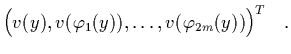
What are the conclusions to be drawn from this theorem? The theorem
considers a time series which is sampled in regular time intervals
as measurements of the observable  at times
  . According
to Takens' theorem one can construct a -dimensional vector
. According
to Takens' theorem one can construct a -dimensional vector
 from the data and this vector is equivalent to the vector
 representing the system on the manifold which contains the
attractor (the attractor is assumed to be simple enough such that it can
be contained in a compact manifold). This equivalence is mathematically
described by the diffeomorphism . So we have
representing the system on the manifold which contains the
attractor (the attractor is assumed to be simple enough such that it can
be contained in a compact manifold). This equivalence is mathematically
described by the diffeomorphism . So we have
(At this stage, we are still restricted to  , but below we will
show that, in fact, nearly every
, but below we will
show that, in fact, nearly every
 can be chosen.)
The difference between Packard's conjecture und Takens' approach is that
Takens requires the embedding space to have a higher dimension
than one would ad hoc expect (). This requirement ensures that
the embedding exists7, but of course it still may be possible to get
reasonable results with a smaller embedding dimension, as one can see
for example from Packard's numerical results.
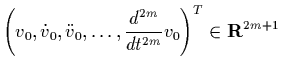
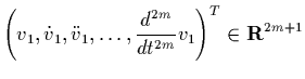
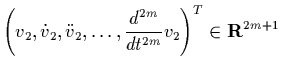
Takens proves two further theorems which give similar results: One of
these theorems justifies the method of delays for maps
(systems defined by eq. (5)) instead of flows (systems like
eq. (1), as considered in the above theorem); the other one
works with embeddings
reconstructed using time derivatives of the observable and corresponds
to Packard's second proposed method (eq. (11)):
In both cases it
is again possible, under genericity assumptions for
can be chosen.)
The difference between Packard's conjecture und Takens' approach is that
Takens requires the embedding space to have a higher dimension
than one would ad hoc expect (). This requirement ensures that
the embedding exists7, but of course it still may be possible to get
reasonable results with a smaller embedding dimension, as one can see
for example from Packard's numerical results.
Takens proves two further theorems which give similar results: One of
these theorems justifies the method of delays for maps
(systems defined by eq. (5)) instead of flows (systems like
eq. (1), as considered in the above theorem); the other one
works with embeddings
reconstructed using time derivatives of the observable and corresponds
to Packard's second proposed method (eq. (11)):
In both cases it
is again possible, under genericity assumptions for  and ,
to embed in -dimensional Euclidean
space8. We have for the derivative method:
and ,
to embed in -dimensional Euclidean
space8. We have for the derivative method:
So both methods suggested by
Packard rather intuitively are hereby justified, although slightly
altered.
With all these theorems one knows how to construct meaningful phase space
vectors from one-dimensional data which has been measured with the
sampling time . This result is interesting but not exhaustive,
because one would like to have the possibility of adjusting  to each
individual situation rather than
having to fix it at some given value; also there is obviously no physical
reason for giving this very special role to the unit time interval. So we
would like to generalize the above result to arbitrary time steps .
Additionally, the important question if one can really reconstruct the
attractor of the dynamical system still remains unanswered. It is
not clear at all that the reconstructed phase space vectors tend to the
same attractor as the picture of the actual flow
to each
individual situation rather than
having to fix it at some given value; also there is obviously no physical
reason for giving this very special role to the unit time interval. So we
would like to generalize the above result to arbitrary time steps .
Additionally, the important question if one can really reconstruct the
attractor of the dynamical system still remains unanswered. It is
not clear at all that the reconstructed phase space vectors tend to the
same attractor as the picture of the actual flow  of
the dynamical system does. For example it could be that the
reconstructed vectors visit only a part of the attractor's equivalent in
. The reason for these doubts is that one is not using
measurements which are made at random times (This would give rise to
the assumption that all these measurements together actually give a true
picture of all parts of the system's trajectory.) but at equidistant times.
So one has to be aware of the possibility that this very special selection
of data points could result in non-equivalence of the original and the
reconstructed attractors.
This uncertainty would mark a fundamental flaw of the attempt to
get a geometrical picture of the attractor, but, fortunately, Takens
provides us here with a theorem, too, which solves both problems.
This theorem (theorem 4 in [4]) says that,
for a compact manifold , a vector field on with the flow
and for , the attractors for the point
of
the dynamical system does. For example it could be that the
reconstructed vectors visit only a part of the attractor's equivalent in
. The reason for these doubts is that one is not using
measurements which are made at random times (This would give rise to
the assumption that all these measurements together actually give a true
picture of all parts of the system's trajectory.) but at equidistant times.
So one has to be aware of the possibility that this very special selection
of data points could result in non-equivalence of the original and the
reconstructed attractors.
This uncertainty would mark a fundamental flaw of the attempt to
get a geometrical picture of the attractor, but, fortunately, Takens
provides us here with a theorem, too, which solves both problems.
This theorem (theorem 4 in [4]) says that,
for a compact manifold , a vector field on with the flow
and for , the attractors for the point  of the
flow and of the mapping
of the
flow and of the mapping
 are the same, generically.
The term ``generically'' refers in this case to the number and
means that the theorem is true for ``almost all'' positive real numbers
. Only for a small subset of
are the same, generically.
The term ``generically'' refers in this case to the number and
means that the theorem is true for ``almost all'' positive real numbers
. Only for a small subset of  the theorem does not hold,
and the probability of choosing ``accidentally'' one of the elements of
this subset is zero.
Thus both of the above problems are solved hereby; the theorem tells us
that we actually can use a time series with a sampling time which we are
free to choose, and despite of the discretization of the original
continuous flow the limit of
the theorem does not hold,
and the probability of choosing ``accidentally'' one of the elements of
this subset is zero.
Thus both of the above problems are solved hereby; the theorem tells us
that we actually can use a time series with a sampling time which we are
free to choose, and despite of the discretization of the original
continuous flow the limit of
 is really equivalent
to the original attractor. So eq. (18) and (19)
hold for nearly all .
Summarizing the results of this section we have seen that,
given a time series of infinite length, one can construct (using e.g.
the method of delays) in practically all cases (i.e. ``generically'')
an infinite series of vectors the limit
set of which is diffeomorphically equivalent to the attractor of the
original dynamical system. The embedding process which gives this result is
summarized in Fig. 4.
is really equivalent
to the original attractor. So eq. (18) and (19)
hold for nearly all .
Summarizing the results of this section we have seen that,
given a time series of infinite length, one can construct (using e.g.
the method of delays) in practically all cases (i.e. ``generically'')
an infinite series of vectors the limit
set of which is diffeomorphically equivalent to the attractor of the
original dynamical system. The embedding process which gives this result is
summarized in Fig. 4.
One has to stress that this result is
somewhat theoretical, since talking about limit sets and attractors
requires an infinitely long time of observation and thus an infinitely
long time series: The last theorem does not give a hint
how many data points or reconstructed phase space vectors one needs to
get an approximation which is ``good'' enough for the ``diffeomorphical
equivalence'' to be true at least approximately. What is more, it is
implicitely assumed that transient initial behaviour has died away and
that the measured time series really corresponds only to phase states
on the attractor. Obviously this can be only an approximation to
any real experimental situation where one will always have
trajectories which are near to the attractor (whatever that means in each
individual case) but not on it. No general information can be given how
long we must
wait to be sure that the the trajectory is near enough to the attractor,
so it is necessary to investigate this problem in each case individually.
Also, the above treatment
implicitely assumes error-free measurements; the accuracy of the time
series is not being questioned but taken for granted. In the next
section, we will deal with these problems in more detail.
Footnotes
- ...
space3
-
For details about Whitney's theorem see e.g. [1].
- ...
4
-
Refer to [2], for example, for a thorough treatment of
embeddings.
- ... conditions5
-
One can interpret the term ``generically'' in this case as follows:
Consider the function space
 of all -functions
which map from into
of all -functions
which map from into  ;
then every subset of consisting only of functions which
do not meet condition (i) and (ii) has zero measure in .
;
then every subset of consisting only of functions which
do not meet condition (i) and (ii) has zero measure in .
- ... well6
-
As hinted by Broomhead and King [7] it is not perfectly
clear on generic grounds that one can exclude solutions with integer periods
: In general one cannot argue that a perturbation of the
generating function will automatically
change the period of the flow. Broomhead and King circumvent this problem
by not considering to be fixed; instead they make it small enough
so that Takens' period-condition is met. See section 3.4.3.
- ... exists7
-
For attractors with a simple geometric structure a smaller embedding
dimension may be sufficient, but the more complicated the structure of
is (e.g. if the attractor is Cantor set-like or if there are many
``backfoldings'') the higher the embedding dimension must be
[5]. The importance of
Takens' result is that, no matter how complex the structure of ,
 dimensions always suffice.
- ...
space8
-
There is one peculiarity for the method using time derivatives: Here,
and must be at least
 -functions, and this
stricter requirement may become a problem if the system or the observable
are not that ``well-behaved''.
-functions, and this
stricter requirement may become a problem if the system or the observable
are not that ``well-behaved''.
Next: Analysis of Real-World Data
Up: Geometry from an Ideal
Previous: The Principle of Reconstruction
Contents
Martin_Engel
2000-05-25