The GOLDBERG Algorithm

In the TROTTER-based algorithm, the position and momentum variables remain nondiscretized; only through the FFT -- which essentially is just a sophisticated formulation of the discrete FOURIER transformation using a discrete set of nodes in position and momentum space -- effectively $x$ and $p$ become discretized, too.

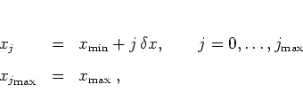
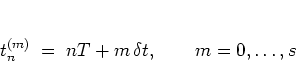
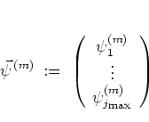
Now I describe a more typical finite differences approach to solving the SCHRÖDINGER equation for the free harmonic oscillator in the position representation, where both space and time are discretized in equidistant steps from the beginning. The solution $\left< x \left\vert \,\psi(t) \right> \right.$ on the interval $[x_{\mbox{\scriptsize min}},x_{\mbox{\scriptsize max}}]$ is constructed at the nodes

$$\begin{array}{lcl} x_j & = & x_{\mbox{\scriptsize min}} + ... ...tsize max}}} & = & x_{\mbox{\scriptsize max}} \; , \end{array}$$ (3.10)

and the time steps

$$t_n^{(m)} \; = \; nT + m \, \delta t, \qquad m=0,\dots,s$$ (3.11)

are used. For simplicity, only the dynamics in the time interval $\big[nT,(n+1)T\big)$ is considered here, such that the subscript $n$ can be dropped. The wave function at site $x_j$ and time $t^{(m)}$, and the potential contribution to $\H_{\mbox{\scriptsize free}}$ at $x_j$ are denoted as

$$\psi_j^{(m)} := % \psi\!\left(x_j,t^{(m)}\right) \left< x_j \left\vert \,\psi\left(t^{(m)}\right) \right> \right.$$ (3.12)

$$v_j \hspace*{0.45cm} := \frac{1}{2}x_j^2,$$ (3.13)

respectively.

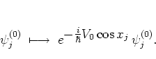
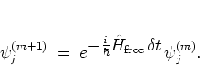
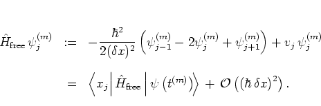
In a first step, ${\hat{U}}_{\mbox{\scriptsize kick}}$ is applied to the discretized wave function:

$$\psi_j^{(0)} \; \longmapsto \; e^{ \textstyle -\frac{i}{\hbar}V_0\cos x_j } \, \psi_j^{(0)} .$$ (3.14)

Then, the new $\psi_j^{(0)}$ is propagated for a period of time of length $T$ using the GOLDBERG algorithm [Koo86,KW96] that I describe now in some more detail.

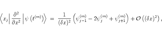
With the discrete first order approximation for the second derivative [SB00]

$$\Big< x_j \Big\vert \,\frac{\partial^2}{\partial x^2}\, \Big... ...+1}^{(m)} \right) + {\mathcal O}\left( (\delta x)^2 \right) ,$$ (3.15)

the application of the free harmonic oscillator Hamiltonian to $\psi_j^{(m)}$ can be written as

$$\begin{array}{lrl} \H_{\mbox{\scriptsize free}}\,\psi_j^{(... ...}\left( \left(\hbar \,\delta x \right)^2 \right) . \end{array}$$ (3.16)

Using this notation, the propagation over the time interval $\delta t$ is approximately

$$\psi_j^{(m+1)} \; = \; e^{ \textstyle -\frac{i}{\hbar}\H_{\mbox{\scriptsize free}} \,\delta t } \, \psi_j^{(m)}.$$ (3.17)

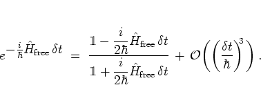
As in the previous subsection it remains to replace the exponential with a suitable approximant, and again using the TAYLOR formula (3.2) is not a good choice, as it does not yield the desired unitary expression. Rather, the GOLDBERG algorithm calls for the CAYLEY form [PTVF94] of the approximant:

$$e^{ \textstyle -\frac{i}{\hbar}\H_{\mbox{\scriptsize free}} ... ... \!\left(\frac{\delta t}{\hbar}\right)^{\!\!\!3} \bigg) \, .$$ (3.18)

Clearly, the quotient on the right hand side is unitary, thereby in principle allowing for an unconditionally stable algorithm. But note that the approximation (3.16) for the application of $\H_{\mbox{\scriptsize free}}$ can still spoil the stability of the algorithm. The CAYLEY approximant is correct up to second order in $\delta t/\hbar$, one power more than would have been supposed at first sight, as both the numerator and the denominator in equation (3.18) are first order approximations only. On the other hand, this very desirable feature of the approximant is accompanied by the less desirable feature that it results in a set of implicit difference equations to be solved -- see equation (3.20) below.

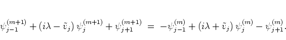
With the abbreviations

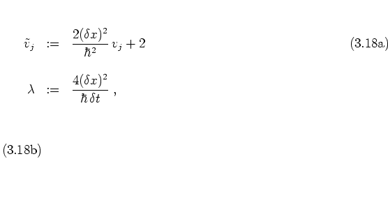
combination of equations (3.16-3.18) gives the iteration scheme

$$\psi_{j-1}^{(m+1)} + \left( i\lambda-\tilde{v}_j \right) \p... ...da+\tilde{v}_j \right) \psi_{j }^{(m )} - \psi_{j+1}^{(m )} .$$ (3.18)

It is to be solved for the $\psi_{j}^{(m+1)}$ and essentially requires the inversion of a tridiagonal system of linear equations. This is seen more easily in vectorial notation. Equation (3.20) is equivalent to

$$A_+\vec{\psi}^{\, (m+1)} \; = \; A_-\vec{\psi}^{\, (m )},$$ (3.19)

for which the vectors

$$\vec{\psi}^{\, (m)} \; := \; \left( \begin{array}{c} \psi... ... \psi_{j_{\mbox{\scriptsize max}}}^{(m)} \end{array} \right)$$ (3.20)

and the symmetric $(j_{\mbox{\scriptsize max}},j_{\mbox{\scriptsize max}})$ matrices

$$A_\pm \; := \; \left( \begin{array}{cccc@{\hspace*{0.4cm}... ...\mp\tilde{v}_{j_{\mbox{\scriptsize max}}} \end{array} \right)$$ (3.21)

have been defined. The value of the parameter $c$ depends on the (DIRICHLET) boundary conditions to be used.

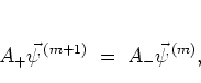
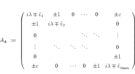
The right hand side of equation (3.21) is easily computed from the already known $\psi_{j}^{(m)}$. Then $\vec{\psi}^{\, (m+1)}=A_+^{-1}A_-\vec{\psi}^{\, (m)}$ is determined by inversion of the (essentially) tridiagonal linear system given by the matrix $A_+$; for that purpose, several efficient algorithms are available [PTVF94,Sto99].

As in the case of the TROTTER-based method, the time increment $\delta t$ can be changed adaptively at each time step in order to control the numerical accuracy of the algorithm. Also, as in the TROTTER algorithm, changing the spatial nodes (and thus $\delta x$) in the course of the calculation is much more difficult and prone to cause additional numerical error.

Regarding the initial choice of the parameters $\delta t$ and $\delta x$, it is natural to choose these parameters small enough such that the smallest oscillation of interest (both with respect to time and space) of the system can be resolved. Furthermore, these parameters can be chosen in such a way that the errors induced by time and space discretization are balanced -- this interdependence is made plausible by equation (3.19b) which shows that reducing $\delta x$ leads to similar numerical problems as increasing $\delta t$; more information on this issue can be found in [KW96] and references therein.