


Next: The GOLDBERG Algorithm
Up: Finite Differences
Previous: Finite Differences
Contents
An Algorithm Based on the TROTTER Formula
Consider the quantum map (2.37).
When discussing states in the position representation,
application of the kick propagator
as in equation (2.34)
is easily accomplished, because
 depends on
  only, and not on
  .
On the other hand, the application of the free propagator,
.
On the other hand, the application of the free propagator,
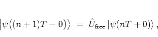 |
(3.1) |
poses a greater problem.
In the form of equation
(2.44)
it is straightforward to let
 act on states expanded
in terms of the harmonic oscillator eigenstates
only -- I come back to this point later in
section 3.3.
For now, I want to discuss the application
of the free propagator to states in the position representation.
act on states expanded
in terms of the harmonic oscillator eigenstates
only -- I come back to this point later in
section 3.3.
For now, I want to discuss the application
of the free propagator to states in the position representation.
Clearly, the exponential
(2.32a)
can be evaluated by expanding it into its
TAYLOR series,
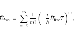 |
(3.2) |
allowing to evaluate
the mapping
(3.1) term by term,
but this approach is problematic from a practical point of view.
Namely, in practice the infinite sum must be truncated at some
finite
value of
 , such that the resulting approximant to the unitary
may become
nonunitary. Unitarity of the propagator
used for the
calculation
is a natural prerequisite for obtaining an
unconditionally stable
[DR96]
numerical algorithm, because in this way conservation of the norm
of the states is automatically built into the method.
Unconditional stability being granted
implies
that the numerical error
-- mainly due to discretization with respect to position and time --
that builds up in the course of many iterations of the quantum map
remains controllable.
, such that the resulting approximant to the unitary
may become
nonunitary. Unitarity of the propagator
used for the
calculation
is a natural prerequisite for obtaining an
unconditionally stable
[DR96]
numerical algorithm, because in this way conservation of the norm
of the states is automatically built into the method.
Unconditional stability being granted
implies
that the numerical error
-- mainly due to discretization with respect to position and time --
that builds up in the course of many iterations of the quantum map
remains controllable.
Therefore, from the point of view of unconditional stability, using a
plain
TAYLOR expansion
should be excluded from the considerations, especially when
it is intended to study
long-time evolution of quantum states.
Nevertheless, in [Dro95]
a procedure is described that allows to
improve on expansions like equation (3.2), but truly
long-time dynamics still seems to remain beyond reach even with this
refined approach.
The basic idea for constructing an unconditionally stable algorithm is
to decompose
into a product where all factors
are already unitary -- and where each factor can be diagonalized by a
suitably simple transformation.
In this way the propagation
over a
full
period  gets replaced with successive propagations over smaller time
steps, such that a discretization with respect to time is introduced into
the method.
gets replaced with successive propagations over smaller time
steps, such that a discretization with respect to time is introduced into
the method.
Above all, the problems with constructing a unitary approximant to
are
caused by the fact that
 is a sum of
two noncommuting
contributions, namely the kinetic and potential terms
is a sum of
two noncommuting
contributions, namely the kinetic and potential terms
 and
and
 .
Since
.
Since
![$[ {\hat{p}}^2, {\hat{x}}^2 ]\neq 0$](img530.png) ,
a simple
BAKER-CAMPBELL-HAUSDORFF (BCH) decomposition
into two unitary factors
is not possible:
,
a simple
BAKER-CAMPBELL-HAUSDORFF (BCH) decomposition
into two unitary factors
is not possible:
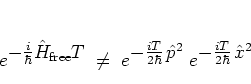 |
(3.3) |
(cf. equation (A.4)
in appendix A
for more on BCH formulae).
An alternative and more suitable approach is based on the
TROTTER product formula.
For two operators  ,
,  and
and
 , the exponential
of the sum of the operators can be expressed as an infinite ordered
product of exponentials of the individual operators:
, the exponential
of the sum of the operators can be expressed as an infinite ordered
product of exponentials of the individual operators:
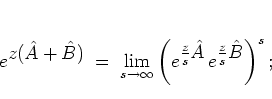 |
(3.4) |
for a proof see [Sch81].
Using the TROTTER formula,
for sufficiently large
 one may approximate:
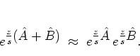 |
(3.5) |
For purely imaginary  ,
the error induced by this approximation,
due to
,
the error induced by this approximation,
due to  being finite,
can be estimated using [DR87]
being finite,
can be estimated using [DR87]
![\begin{displaymath}
\bigg\Vert \,
e^{\textstyle \frac{z}{s}({\hat{A}}+{\hat{B}}...
...2s^2} \,
\left\Vert \, [{\hat{A}},{\hat{B}}] \, \right\Vert ,
\end{displaymath}](img539.png) |
(3.6) |
where  is a suitable operator norm.
Note that, using the estimate (3.6),
for commuting
is a suitable operator norm.
Note that, using the estimate (3.6),
for commuting
 the simplest BCH result
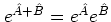 is confirmed again.
In the present context of the kicked harmonic oscillator,
I obtain the following approximation for the free propagator,
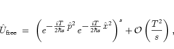 |
(3.7) |
which can be made as accurate as desired by increasing .
Note that the upper bound of the error does not depend explicitly on
 any more, such that the quality of the algorithm, as given
by the error term
any more, such that the quality of the algorithm, as given
by the error term
 , does not vary with .
Unitarity of the approximating propagator is granted by
, does not vary with .
Unitarity of the approximating propagator is granted by
 ,
,  being Hermitian.
As opposed to
in the form of equation (3.2),
application of its approximant (3.7) is
straightforward.
For each of the time steps per period ,
expressions of the following type have to be evaluated:
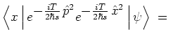 |
|
|
(3.8) |
| |
|
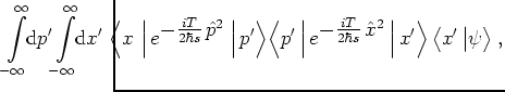 |
|
i.e. the -dependent exponential is multiplied to the initial state
in the position representation, the result is transformed into the
momentum representation, where the -dependent exponential is
easily applied; finally, the resulting expression is transformed back into
the position representation.
In this way, the free harmonic oscillator dynamics of arbitrary states
is obtained
essentially
by successively switching between the position and momentum
representations; this can be done quite effectively using the
technique of
fast FOURIER transformation (FFT)
[CT65,EMR93].
Nevertheless, the
need for applying the FFT very often
in order to obtain the desired accuracy is the limiting bottleneck for
this
algorithm.3.1
The full kicked harmonic oscillator
dynamics is then obtained by
alternately applying the simple
of equation
(2.34) and the TROTTER-approximated
as described above.
Effectively, the TROTTER algorithm
implies
a discretization of
the dynamics with respect to time; the period of time of the
unperturbed harmonic oscillator dynamics is split into sufficiently
small time steps of length
 |
(3.9) |
This may be used to implement an adaptive step size control:
each time the approximate propagator (3.7) is applied,
can be tuned to be small enough to make the algorithm not too
time-consuming on the one hand, and large enough to achieve the desired
accuracy on the other hand;
the latter can be checked by applying (3.7) twice each
time, for example using and  , and comparing the two resulting
iterated states.
(The same applies to the number of nodes used
for storing
, and comparing the two resulting
iterated states.
(The same applies to the number of nodes used
for storing
 and
and
 , but in contrast
to this number cannot be changed easily in the course of the
calculation, but rather has to be specified before the algorithm is
started.)
, but in contrast
to this number cannot be changed easily in the course of the
calculation, but rather has to be specified before the algorithm is
started.)
Footnotes
- ...
algorithm.3.1
- In [See95] a stroboscopically kicked
(and otherwise free) particle is studied
quantum mechanically using a similar algorithm
of successive transformations between the position
and momentum representations
(with modifications as described in
[HM87]
which
regrettably
are not applicable to
the present case of the cosine kicked harmonic
oscillator
where the kick potential is not of finite range).
Similarly, in subsection 5.1.1 and
in [Lan94] the quantum dynamics of the
cosine-kicked rotor is discussed.
In
these systems,
only a single
pair of FOURIER transformations per kick period is
needed, because between the kicks the (free)
dynamics in the momentum representation is trivial.
The present subsection 3.1.1
illustrates the way in which
the situation becomes considerably more intricate when
replacing the truly free
dynamics between the kicks with the ``free''
harmonic oscillator dynamics.
Next: The GOLDBERG Algorithm
Up: Finite Differences
Previous: Finite Differences
Contents
Martin Engel 2004-01-01