In this section I discuss some of the aspects of the practical implementation of the iteration scheme outlined in subsection 2.1.3.
From a formal point of view
the methods
formulating ![]() in
the position representation
(section 3.2)
and the eigenrepresentation of the harmonic oscillator
(subsection 2.1.3 and the present section)
obviously are very similar
-- for example, both equation (2.43) and
equation (3.28)
are
explicit
linear mappings of vectors of complex numbers.
in
the position representation
(section 3.2)
and the eigenrepresentation of the harmonic oscillator
(subsection 2.1.3 and the present section)
obviously are very similar
-- for example, both equation (2.43) and
equation (3.28)
are
explicit
linear mappings of vectors of complex numbers.
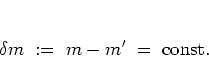
What is more, the dimensions of the matrices ![]() and
and
![]() used for the iterations are of the same order of magnitude, too.
This can be seen as follows.
The dimension
used for the iterations are of the same order of magnitude, too.
This can be seen as follows.
The dimension
![]() to be used for
to be used for
![]() has been
derived in the previous subsection; on the other hand,
the dimension needed for
has been
derived in the previous subsection; on the other hand,
the dimension needed for ![]() is determined by the maximum index
is determined by the maximum index
![]() of the set
of the set
![]() necessary for resolving quantum phase space structures at a distance of
necessary for resolving quantum phase space structures at a distance of
![]() from the origin.
Roughly speaking,
from the origin.
Roughly speaking,
![]() is peaked
around the
corresponding
classical turning points at
is peaked
around the
corresponding
classical turning points at
![]() and decays
exponentially
for larger values of
and decays
exponentially
for larger values of
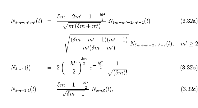
![]() .3.2This means that, as a rule of the thumb,
the dimension of
.3.2This means that, as a rule of the thumb,
the dimension of ![]() needed for describing the dynamics on the interval
needed for describing the dynamics on the interval
![]() is not very much larger than
is not very much larger than
![]() . This estimate is
close to the value of
. This estimate is
close to the value of
![]() determined in
equation (3.32).
determined in
equation (3.32).
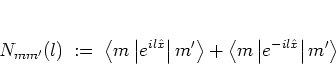
There are some decisive differences between the matrices used for the
two methods, as well.
First of all,
with respect to identical dimensions of the matrices,
storing the matrix elements of ![]() only requires a quarter
of the memory needed for storing the matrix elements of
only requires a quarter
of the memory needed for storing the matrix elements of
![]() :
in practice, the kick matrix elements
:
in practice, the kick matrix elements ![]() of equation (2.51)
-- rather than the
full FLOQUET matrix elements
of equation (2.51)
-- rather than the
full FLOQUET matrix elements ![]() -- are stored in the computer
memory, such that the selection rule
-- are stored in the computer
memory, such that the selection rule ![]() for
for ![]() odd and the
symmetry property
odd and the
symmetry property
![]() can be used
-- see equation (2.51).
Then, each time they are needed during the iteration,
the
can be used
-- see equation (2.51).
Then, each time they are needed during the iteration,
the ![]() are trivially calculated from the
are trivially calculated from the ![]() using the
splitting (2.45).
Storing the
using the
splitting (2.45).
Storing the ![]() requires computer memory for roughly
requires computer memory for roughly
![]() complex numbers, i.e. for the typical value of
complex numbers, i.e. for the typical value of
![]() some 138 MBytes are needed. The
approximate
CPU time per iteration of the quantum map then typically varies
from 45 sec (on a Pentium II with 350 MHz)
to 10 sec (Pentium 4 with 2 GHz).
some 138 MBytes are needed. The
approximate
CPU time per iteration of the quantum map then typically varies
from 45 sec (on a Pentium II with 350 MHz)
to 10 sec (Pentium 4 with 2 GHz).
Second,
in contrast
to the evaluation of (3.30),
computation of the ![]() and thus of the
and thus of the ![]() is a nontrivial
task.
Equation (2.51) shows that the formula
for the
is a nontrivial
task.
Equation (2.51) shows that the formula
for the ![]() is
composed of several terms (BESSEL functions,
generalized LAGUERRE polynomials,
factorials, exponentials) the
absolute values
of which can -- and in practice do
-- differ greatly, such that all kinds of numerical cancellations,
overflows and underflows are to be expected -- and indeed do occur --
when (2.51) is evaluated directly.
Therefore, this calculation has to be implemented in a slightly more
sophisticated way, basically by exploiting the recurrence relation
is
composed of several terms (BESSEL functions,
generalized LAGUERRE polynomials,
factorials, exponentials) the
absolute values
of which can -- and in practice do
-- differ greatly, such that all kinds of numerical cancellations,
overflows and underflows are to be expected -- and indeed do occur --
when (2.51) is evaluated directly.
Therefore, this calculation has to be implemented in a slightly more
sophisticated way, basically by exploiting the recurrence relation
for the generalized LAGUERRE polynomials [AS72].
In this way, not only the abovementioned numerical problems are avoided,
but also the computation of the whole matrix is sped up considerably.
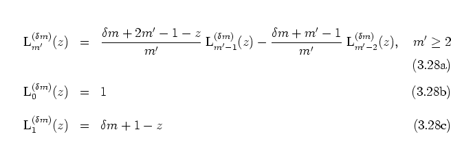
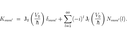
Starting from the kick matrix elements in the form of equation
(2.48) and using the definition
 |
(3.28) |
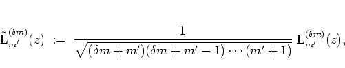
The matrix elements ![]() in this expression need to be studied
with respect to their behaviour along the diagonals given by
in this expression need to be studied
with respect to their behaviour along the diagonals given by
 |
(3.30) |
The
![]() can now be calculated efficiently using the
recurrence relation
can now be calculated efficiently using the
recurrence relation
which is obtained by evaluating the
 in equation (3.38) by means of the definition
(3.37) and the recursion relation
(3.33) of the generalized LAGUERRE polynomials.
in equation (3.38) by means of the definition
(3.37) and the recursion relation
(3.33) of the generalized LAGUERRE polynomials.
The numerical problems mentioned above with respect to the direct evaluation of equation (2.51) are reduced to a minimum with this algorithm, because multiplying and adding up very large and very small numbers at the same time is avoided here as far as possible: the definition (3.37) avoids the factorials of equation (2.51), and the respective absolute values of the numerators and denominators in each of the fractions in the recursion (3.39a) are constructed to be as comparable as possible.
Similarly, when
in the next chapters
![]() needs to be evaluated
numerically
for larger values
of
needs to be evaluated
numerically
for larger values
of ![]() ,
this cannot be done
using
equation (2.39) directly. Rather, a
scaled variant
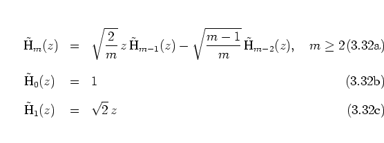
of the HERMITE polynomials is defined,
,
this cannot be done
using
equation (2.39) directly. Rather, a
scaled variant
of the HERMITE polynomials is defined,
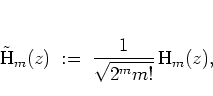 |
(3.32) |
![\begin{subequations}
\begin{eqnarray}
{\mbox{H}}_m(z)
& = & 2z \, {\mbox{H}}_{...
...cm]
{\mbox{H}}_1(z) \hspace*{0.11cm}
& = & 2z
\end{eqnarray}\end{subequations}](img637.png)
 |
(3.31) |
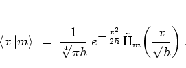
With the
![]() computed
as described above,
the series in equation (3.35) can be evaluated term by term.
In the parameter range considered for the numerical calculations
in the following chapters, the series
can
typically be truncated at values of
computed
as described above,
the series in equation (3.35) can be evaluated term by term.
In the parameter range considered for the numerical calculations
in the following chapters, the series
can
typically be truncated at values of ![]() not exceeding 200, while
keeping the error induced by the truncation reasonably small.
(For the maximum relative error due to this truncation,
not exceeding 200, while
keeping the error induced by the truncation reasonably small.
(For the maximum relative error due to this truncation, ![]() was a
somewhat typical value in the practical calculations.)
was a
somewhat typical value in the practical calculations.)
As in the previous sections,
boundary conditions
have to be imposed here, too. After each time step it is checked if the
condition (3.24a) is still satisfied. In practice, for
diffusing states violation of this boundary condition
-- due to the implicit cut-off error as a result of the finite number
![]() of basis elements
of basis elements
![]() used for expanding the states
--
is one of the two main sources of numerical error. The other is the
unavoidable
rounding error
generated in the course of the
numerical
computation
of the
used for expanding the states
--
is one of the two main sources of numerical error. The other is the
unavoidable
rounding error
generated in the course of the
numerical
computation
of the ![]() .
.
![\begin{displaymath}
N_{\delta m+m',m'}(l)
\; = \; \displaystyle
\left\{ \dis...
... m$\ odd.
\rule[-0.3cm]{0.0cm}{0.3cm}
}
\end{array} \right.
\end{displaymath}](img624.png)