In [BR95] a numerical ``brute force approach'' to
determining the kicked harmonic oscillator dynamics is described.
Using the present terminology and scaling, this approach
can be formulated as a
discretization of the
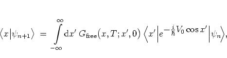
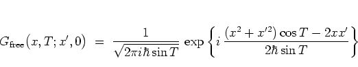
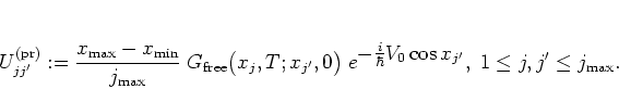
integral form of the quantum map (2.37)
in the position representation,
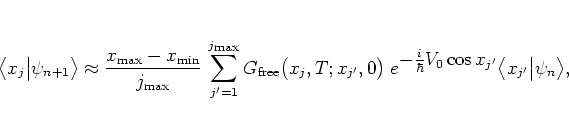
Using the ![]() -discretization
as given by equations
(3.10), the integral expression (3.25)
can be approximated by
-discretization
as given by equations
(3.10), the integral expression (3.25)
can be approximated by
 |
(3.25) |
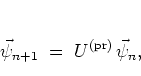
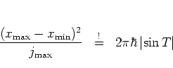
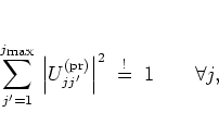
In order to obtain a numerically stable algorithm,
![]() must be required to be unitary,
must be required to be unitary,
 |
(3.27) |
In addition to the condition
(3.32),
a boundary condition of the type (3.24a)
also
needs
to be satisfied, i.e. the interval
![]() must be chosen large enough to
allow the discrete mapping (3.27) to approximate the
original
(3.25) well enough. This is granted if the wave function
must be chosen large enough to
allow the discrete mapping (3.27) to approximate the
original
(3.25) well enough. This is granted if the wave function
![]() decays rapidly enough with
decays rapidly enough with ![]() reaching out to the
boundaries of the interval considered.
reaching out to the
boundaries of the interval considered.
These two restrictions combined are the reason why the algorithm given
by the mapping (3.27)
is of
limited
practical use when the long-time dynamics of
spreading states
is to be studied:
for delocalized states spreading widely along the ![]() -axis, very large
values of
-axis, very large
values of
![]() are required by the
condition (3.32),
in particular when
are required by the
condition (3.32),
in particular when ![]() takes on small values.
This means that the memory requirements on the computer
grow rapidly,
and the evaluation of each iteration of (3.27) quickly
becomes more time-consuming.
For example, the
values
takes on small values.
This means that the memory requirements on the computer
grow rapidly,
and the evaluation of each iteration of (3.27) quickly
becomes more time-consuming.
For example, the
values
![]() ,
,
![]() and
and ![]() lead to
lead to
![]() ,
making it practically impossible
to store the matrix elements
,
making it practically impossible
to store the matrix elements
![]() on a typical workstation and
slowing down the speed of the computation
considerably.
It is important to keep in mind this limitation of the algorithm when
working with it in practice.
on a typical workstation and
slowing down the speed of the computation
considerably.
It is important to keep in mind this limitation of the algorithm when
working with it in practice.
Conversely, if the dynamics is followed for times ![]() not too large,
such that the initial wave packets have not spread too much,
then equation (3.27) provides a simple and efficient
way to evaluate the quantum map (2.37),
especially for larger values of
not too large,
such that the initial wave packets have not spread too much,
then equation (3.27) provides a simple and efficient
way to evaluate the quantum map (2.37),
especially for larger values of ![]() .
.