An important subject in solid state physics is the investigation of electronic motion in disordered solids at low temperature. ANDERSON initiated a particular type of research in this field, focusing on one-dimensional lattices as model systems for the crystal lattices of solids [And58,And61,And78]. (A more recent review may be found in [LR85].) Here, I discuss only those aspects of the theory that are relevant for the understanding of localization phenomena on such lattices that can be taken as simple model systems for disordered solids.
The concept of transfer matrices [Pen94] is an essential
ingredient of
the theory. As an introductory example for the use of these matrices I
consider a simplified discussion of
a stationary quantum wave function within
the one-dimensional
potential
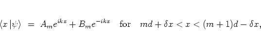
In the zero potential region
between the ![]() -st and
-st and ![]() -th site
the
quantum
wave function can be written in the
form
-th site
the
quantum
wave function can be written in the
form
 |
(5.8) |
 |
(5.10) |
 |
(5.11) |
For a periodic potential
![]() with
with
![]() the conditions for complete
transmission through a lattice site are identical for all sites and can
be satisfied by adjusting the energy of the
electron.
This is
a consequence
of BLOCH's theorem which asserts the existence of delocalized
motion [Mad78].
the conditions for complete
transmission through a lattice site are identical for all sites and can
be satisfied by adjusting the energy of the
electron.
This is
a consequence
of BLOCH's theorem which asserts the existence of delocalized
motion [Mad78].
For aperiodic potentials, on the other hand,
which -- as discussed above -- provide a more appropriate model for
disordered solids than periodic potentials, the situation is
different and more conveniently discussed in terms of
another
class of
systems,
giving rise to another type of transfer matrices.
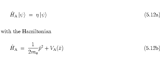
Here, the role of the
time-independent SCHRÖDINGER equation
is taken by
the discrete SCHRÖDINGER equation
[And58,And78]:
The discrete SCHRÖDINGER equation (5.20) can
be derived from its continuous counterpart, the time-independent
SCHRÖDINGER equation for a state
![]() with energy
with energy ![]() ,
,
and the electron mass
![]() ,
in the following way.
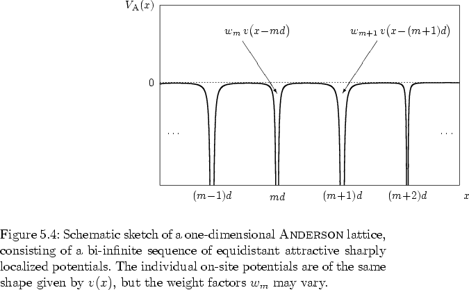
The potential (5.15)
again
has been
assumed to be composed
of well localized, nonoverlapping individual potentials
,
in the following way.
The potential (5.15)
again
has been
assumed to be composed
of well localized, nonoverlapping individual potentials ![]() . This
assumption is often called the
tight binding approximation(see for example [Stö99])
-- although some authors also refer to tight binding
with respect to
a special case
of the model that I
discuss
below on page
. This
assumption is often called the
tight binding approximation(see for example [Stö99])
-- although some authors also refer to tight binding
with respect to
a special case
of the model that I
discuss
below on page ![[*]](crossref.png) .
.
Let the eigenstates of ![]() be denoted by
be denoted by
![]() ,
with
,
with ![]() labelling the different eigenstates.
While a general state needs to be constructed by superposition of all of
these
labelling the different eigenstates.
While a general state needs to be constructed by superposition of all of
these
![]() , for the model system to be discussed here
it suffices to consider a single eigenstate,
, for the model system to be discussed here
it suffices to consider a single eigenstate,
![]() ,
taken to be normalized.
It may be looked upon as that single atom state interacting strongest
with the passing electron.
Obviously, the restriction to a single eigenstate is a further assumption
on the system, but allowed in the present context, since the resulting
model system is still powerful enough to explain some of the key features
of electronic states in disordered crystalline lattices.
The localization property of
,
taken to be normalized.
It may be looked upon as that single atom state interacting strongest
with the passing electron.
Obviously, the restriction to a single eigenstate is a further assumption
on the system, but allowed in the present context, since the resulting
model system is still powerful enough to explain some of the key features
of electronic states in disordered crystalline lattices.
The localization property of ![]() carries over to
carries over to
![]() ,
such that the following
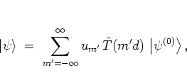
LCAO ansatz (linear combination of atomic orbitals, [Zim79])
for an eigenstate
,
such that the following
LCAO ansatz (linear combination of atomic orbitals, [Zim79])
for an eigenstate
![]() of the
complete lattice can
be made,
of the
complete lattice can
be made,
Inserting
the expansion
(5.22) into
the SCHRÖDINGER equation
(5.21),
and making use of the orthonormality relation
 |
(5.15) |
 |
(5.16) |
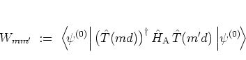
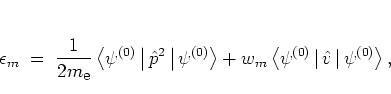
Essentially, the expectation values ![]() , taken with respect to
, taken with respect to
![]() , depend
on the weight factors
, depend
on the weight factors ![]() of
of
![]() only,
only,
Up to this point,
the dynamics on the lattice as given by equation
(5.20)
is completely deterministic, and its
parameters are all fixed by specifying
![]() .
On the other hand, since
a priori
the eigenstates
.
On the other hand, since
a priori
the eigenstates
![]() are unknown
and the calculation of the
are unknown
and the calculation of the ![]() and
and ![]() might be
a difficult task, it is much simpler to choose these quantities in
an appropriate way, making the model as simple as possible, while still
retaining its essential characteristics.
In the following I
discuss the most important of the possible choices, which is known as
diagonal or site disorder.
Here, the matrix elements
might be
a difficult task, it is much simpler to choose these quantities in
an appropriate way, making the model as simple as possible, while still
retaining its essential characteristics.
In the following I
discuss the most important of the possible choices, which is known as
diagonal or site disorder.
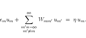
Here, the matrix elements
![]() are assumed to be ``constant'', i.e. they are not treated as
varying much with
are assumed to be ``constant'', i.e. they are not treated as
varying much with ![]() ,
, ![]() . Frequently, most of the
. Frequently, most of the ![]() are taken
to be zero, and
just
a few of them take on a very limited number of
nontrivial values. A typical example for such a choice is given below in
equation (5.30). The disorder part of
the case of site disorder is constituted by assuming the diagonal energies to vary
with
are taken
to be zero, and
just
a few of them take on a very limited number of
nontrivial values. A typical example for such a choice is given below in
equation (5.30). The disorder part of
the case of site disorder is constituted by assuming the diagonal energies to vary
with ![]() , in such a way that the
, in such a way that the ![]() are statistically distributed
according to a given distribution and nothing more is known about them.
It is a nice feature of this particular model that,
as indicated by
equation
(5.27), the assumptions concerning the distribution
of the
are statistically distributed
according to a given distribution and nothing more is known about them.
It is a nice feature of this particular model that,
as indicated by
equation
(5.27), the assumptions concerning the distribution
of the ![]() carry over to the
carry over to the ![]() , and vice versa. In this way
it is possible to adjust the disorder properties of the model by
specifying the weight factors of
the ``random potential''
, and vice versa. In this way
it is possible to adjust the disorder properties of the model by
specifying the weight factors of
the ``random potential''
![]() in the very
beginning of the
discussion.5.5
in the very
beginning of the
discussion.5.5
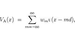
Often, the model potential
![]() is defined in such a
way that the resulting discrete SCHRÖDINGER equation is at least
approximately translation invariant
with the lattice constant
is defined in such a
way that the resulting discrete SCHRÖDINGER equation is at least
approximately translation invariant
with the lattice constant ![]() ,
i.e. the matrix elements
,
i.e. the matrix elements ![]() depend on the distance of the two respective sites
depend on the distance of the two respective sites ![]() and
and ![]() only.
In these cases
the simplified discrete SCHRÖDINGER equation
only.
In these cases
the simplified discrete SCHRÖDINGER equation
Depending on
![]() , the model may be simplified even
further.
In order to study ANDERSON localization it suffices to consider the
special case
where only the interaction with nearest neighbours is taken into account
and assumed to be symmetric,
, the model may be simplified even
further.
In order to study ANDERSON localization it suffices to consider the
special case
where only the interaction with nearest neighbours is taken into account
and assumed to be symmetric,
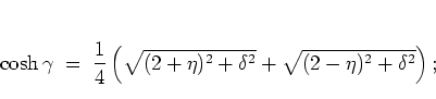
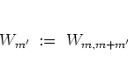
![\begin{subequations}
\begin{eqnarray}
W_{m'} \hspace*{-0.1cm}
& = & \! 0 \quad...
...0.2cm]
W_{-1} \hspace*{-0.15cm}
& = & \! W_1.
\end{eqnarray}\end{subequations}](img978.png)
The restriction (5.30a)
is also frequently referred to as the tight binding
approximation [Fis93].
(Cf. the discussion of tight binding on page
.)
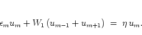
The resulting tight binding equation is
Again, this time as a result of the tight binding approximation
(5.30a),
the problem can be formulated using
a
transfer matrix approach
by setting
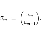
Every point
(here: corresponding to the index ![]() )
to the right of some initial point
(with index
)
to the right of some initial point
(with index ![]() )
on the lattice
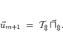
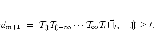
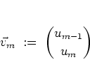
can be reached by repeated application of the transfer matrix:
)
on the lattice
can be reached by repeated application of the transfer matrix:
In such a setting FURSTENBERG's theorem
[Fur63]
can be applied, which deals with the more general class of unimodular
random matrices. Obviously the ![]() are unimodular for all
are unimodular for all ![]() ,
,
 |
(5.26) |
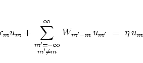
A necessary condition for this explanation to work is that the diagonal
energies ![]() are randomly distributed under variation of
are randomly distributed under variation of ![]() .
The
definition of a
tight binding model thus has to be completed by specifying the
distribution function
.
The
definition of a
tight binding model thus has to be completed by specifying the
distribution function ![]() for the
values of
for the
values of
![]() .
Actually, in order to ensure that FURSTENBERG's theorem is
applicable,
.
Actually, in order to ensure that FURSTENBERG's theorem is
applicable, ![]() must be ``sufficiently well-behaved'' in a
way that is described in some more detail in appendix
B.
(In [FMSS85,CKM87]
ANDERSON localization is even proved under assumptions which are
somewhat weaker than those of FURSTENBERG's theorem, as discussed in
appendix B.)
Several different choices for
must be ``sufficiently well-behaved'' in a
way that is described in some more detail in appendix
B.
(In [FMSS85,CKM87]
ANDERSON localization is even proved under assumptions which are
somewhat weaker than those of FURSTENBERG's theorem, as discussed in
appendix B.)
Several different choices for ![]() satisfying these
requirements
have been applied successfully;
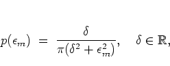
choosing a
Lorentzian distribution function -- in which case the model is
often referred to as the ANDERSON-LLOYD model --,
satisfying these
requirements
have been applied successfully;
choosing a
Lorentzian distribution function -- in which case the model is
often referred to as the ANDERSON-LLOYD model --,
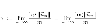
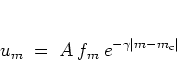
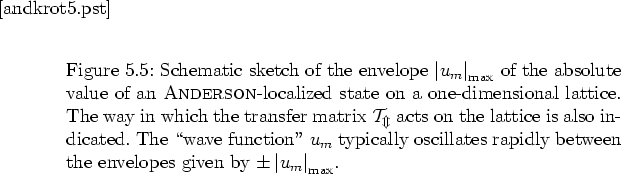
To summarize, a discrete SCHRÖDINGER equation describing electronic motion within the framework of a one-dimensional lattice model of a disordered solid has been derived, and I have demonstrated that typical solutions exhibit exponential localization.
![\begin{displaymath}
\cal{T}_m
\; = \; \left( \begin{array}{cc}
\eta-\epsilon_m & -1 \\ [0.2cm]
1 & 0
\end{array} \right),
\end{displaymath}](img983.png)