Mapping of the Quantum Kicked Rotor onto the
ANDERSON Model

Combining the results of the two preceding subsections, I now present the argument showing that the quantum kicked rotor exhibits ANDERSON localization, by deriving a mapping of the rotor model onto the ANDERSON model [FGP82,GFP82,PGF83].

I begin this discussion of the quantum map (5.8) with a general kick potential $V(\vartheta)$,

$$\left\vert \psi_{n+1} \right> \; = \; e^{\textstyle -\frac... ...-\frac{i}{\hbar}V(\hat{\vartheta})} \left\vert \psi_n \right>,$$ (5.31)

and specialize to particular potentials -- the cosine potential (5.2) being one of two to be considered -- later in the course of the discussion. Using the results of subsection 2.1.1, $\left\vert \psi_n \right>$ can be expanded in terms of the quasienergy states of the kicked rotor $\left\vert \phi_E(t) \right>$ with constant coefficients $A_E$:

$$\left\vert \psi_n \right> \; = \; \sum_E A_E \left\vert \phi_E(n) \right>.$$ (5.32)

Since the $A_E\in\mathbb{C}$ are time-independent it suffices to consider in the following the time evolution of a single quasienergy state rather than the general $\left\vert \psi_n \right>$ of equation (5.44).

For the investigation of the kicked rotor the states $\left\vert u_E(t) \right>$ are much better suited than the full quasienergy states $\left\vert \phi_E(t) \right>$, since by the periodicity (2.24) the time argument can be dropped altogether. This allows to map the dynamical system (5.43) onto a static problem. In accordance with the discrete nature of the kick, I define the (reduced) quasienergy states immediately before and after the kicks as

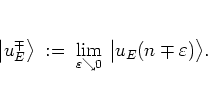$$\left\vert u_E^\mp \right> \; := \; \lim_{\varepsilon\searrow 0} \, \big\vert u_E(n\mp \varepsilon) \big>.$$ (5.33)

In terms of the new states the quantum map can now be formulated as

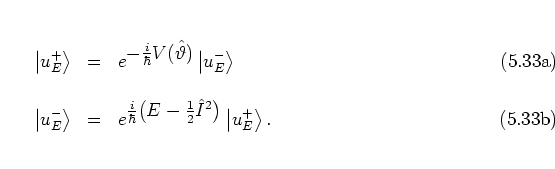
It turns out that the kick part (5.46a) of the dynamics is most conveniently described using the averaged state

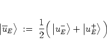$$\big\vert \overline{u}_E \big> \; := \; \frac{1}{2} \Big( \left\vert u_E^- \right>+\left\vert u_E^+ \right> \Big)$$ (5.33)

and exchanging the potential $V(\hat{\vartheta})$ for the expression

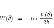$$W(\hat{\vartheta}) \; := \; -\tan \frac{V(\hat{\vartheta})}{2\hbar}.$$ (5.34)

This definition of $W(\hat{\vartheta})$ can be used to rewrite the kick propagator as

$$e^{\textstyle -\frac{i}{\hbar}V(\hat{\vartheta})} \; = \; \frac{1+iW(\hat{\vartheta})}{1-iW(\hat{\vartheta})},$$ (5.35)

such that I obtain by substitution into equation (5.46a):

Inserting these expressions into the equation (5.46b) that describes the free part of the dynamics, the $\left\vert u_E^\mp \right>$ are eliminated from the equation and the dynamics is entirely formulated in terms of the averaged quasienergy state $\big\vert \overline{u}_E \big>$:

$$\left(1-iW(\hat{\vartheta})\right) \big\vert \overline{u}_E ... ...t(1+iW(\hat{\vartheta})\right) \big\vert \overline{u}_E \big>.$$ (5.35)

In order to facilitate the evaluation of the action of the angular momentum operator $\hat{I}$, this equation is projected onto the eigenstates $\left\vert m \right>_{\rm r}$ of $\hat{I}$ (see equation (5.12)). To this end I define

$$\overline{u}_{E,m} \; := \; \rule[-0.1cm]{0.0cm}{0.1cm}_{\... ...left\vert \overline{u}_E \right> \right., \quad m\in\mathbb{Z}$$ (5.36)

and obtain

$$\tan \left( \frac{1}{2\hbar} \left( E-\frac{\hbar^2m^2}{2}... ... m \big\vert \hat{W} \big\vert \overline{u}_E \big> \; = \; 0.$$ (5.37)

It remains to evaluate the matrix element $\rule[-0.1cm]{0.0cm}{0.1cm}_{\rm r} \big< m \big\vert \hat{W} \big\vert \overline{u}_E \big>$. By virtue of the representation (5.12) of $\left\vert m \right>_{\rm r}$ it is easily seen that the matrix element $\rule[-0.1cm]{0.0cm}{0.1cm}_{\rm r} \big< m \big\vert \hat{W} \big\vert m' \big>_{\rm r}$ satisfies

$$\rule[-0.1cm]{0.0cm}{0.1cm}_{\rm r} \big< m \big\vert \hat{... ...hat{W} \big\vert 0 \big>_{\rm r} \; , \quad m'\in\mathbb{Z},$$ (5.38)

i.e. the matrix element depends on the difference of the quantum numbers $m$, $m'$ only. Therefore it makes sense to use just a single index $m'$ and define the ``interaction energy'' as^5.7

$$W_{m'} \; := \; % \frac{1}{\sqrt{2\pi}} \, \rule[-0.1cm]{0... ...rt \hat{W} \big\vert 0 \big>_{\rm r}, % \; , \quad m'\in\ZZ,$$ (5.39)

in terms of which the matrix element $\rule[-0.1cm]{0.0cm}{0.1cm}_{\rm r} \big< m \big\vert \hat{W} \big\vert \overline{u}_E \big>$ reads:

$$\rule[-0.1cm]{0.0cm}{0.1cm}_{\rm r} \big< m \big\vert \hat... ...sum_{m'=-\infty}^\infty \, W_{m'} \, \overline{u}_{E,m-m'}\; .$$ (5.40)

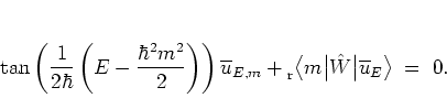
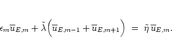
In the end one thus arrives at an equation analogous to the discrete SCHRÖDINGER equation (5.20) with $\eta=0$,

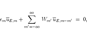$$\epsilon_m \overline{u}_{E,m} + \sum_{m'=-\infty}^\infty \, W_{m'} \, \overline{u}_{E,m-m'} \; = \; 0,$$ (5.41)

with the diagonal energies $\epsilon_m\in\mathbb{R}$ given by

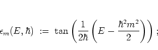$$\epsilon_m(E,\hbar) \; := \; \tan \left( \frac{1}{2\hbar} \left( E-\frac{\hbar^2m^2}{2} \right) \right);$$ (5.42)

the hopping matrix elements $W_{m'}$ describe the coupling of a ``site of the lattice'' $\{\overline{u}_{E,m}\}$ with its $m'$-th nearest neighbour, due to the kick. By the property (5.54) this coupling depends on the distance between the two sites only, which means that the system is translation invariant.

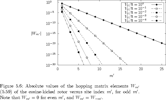
Note that in general equation (5.57) is not a tight binding equation (5.31), since the interaction is not restricted to just the respective nearest neighbours of each site. In fact, the cosine potential (5.2) leads to

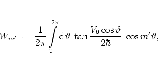$$W_{m'} \; = \; \frac{1}{2\pi} \int\limits _0^{2\pi} {\mbox{... ...ar}. \tan\frac{V_0\cos\vartheta}{2\hbar} \; \cos m'\vartheta,$$ (5.43)

which implies that $W_{m'}=0$ for even $m'$, but also that, generally speaking, all $W_{m'}$ for odd $m'$ are possibly nonzero. Nevertheless, for this cosine potential $W_{m'}$ decays rapidly -- obviously exponentially -- with $m'$, as figure 5.7 shows, where $\vert W_{m'}\vert$ (obtained by numerical evaluation of the integral in equation (5.59), since a closed formula for this integral is lacking) as a function of $m'$ is plotted for several parameter combinations.

The figure indicates that the corresponding discrete SCHRÖDINGER equation (5.57), while not exactly describing a tight binding model, is a good approximation to a tight binding equation for suitable combinations of the parameters $V_0$, $\hbar$. Namely, equation (5.57) becomes a true tight binding equation in the limit $V_0/\hbar\to 0$, i.e. for weak perturbations and/or in the fully quantum mechanical regime specified by large values of $\hbar$. The tight binding system

$$\epsilon_m \overline{u}_{E,m} + W_1\left( \overline{u}_{E,m-1} +\overline{u}_{E,m+1} \right) \; = \; 0$$ (5.44)

obtained in this limit can be described -- in analogy to the transfer matrix (5.33) in ANDERSON's theory -- by the transfer matrix^5.8

$$\cal{T}_m \; = \; \left( \begin{array}{cc} \displaystyle ... ...silon_m}{W_1}\;\; & -1 \\ [0.5cm] 1 & 0 \end{array} \right),$$ (5.45)

acting on the vectors

via

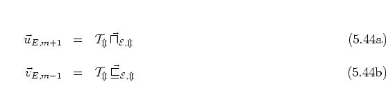
-- cf. the vectors (5.32, 5.36) and the ``equations of motion'' (5.34, 5.37) of the ANDERSON model in subsection 5.1.2.

By choosing a different kick potential $V(\vartheta)$ the transition to a true tight binding model may be achieved. The choice of the potential affects the hopping matrix elements only and leaves the diagonal energies unchanged. For the alternate potential

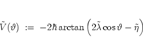$$\tilde{V}(\vartheta) \; := \; -2\hbar \arctan \left( 2\tilde{\lambda}\cos\vartheta-\tilde{\eta} \right)$$ (5.44)

with arbitrary real constants $\tilde{\eta}$ and $\tilde{\lambda}\neq 0$, the corresponding alternate hopping matrix elements are

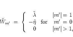$$\tilde{W}_{m'} \; = \; \left\{ \begin{array}{rcr@{}c@{}l@... ... 0 & & \vert&m'&\vert & \, > \, & \, 1, \end{array} \right.$$ (5.45)

such that with this potential one gets a tight binding model without having to rely on an approximation:

$$\epsilon_m \overline{u}_{E,m} + \tilde{\lambda} \Big( \ove... ...{u}_{E,m+1} \Big) \; = \; \tilde{\eta} \, \overline{u}_{E,m}.$$ (5.46)

For all practical purposes the diagonal energies $\epsilon_m$ of (5.58) can be taken to be randomly distributed as in the ANDERSON-LLOYD model, which can be seen as follows. In the absence of the quantum resonances [Fis93] defined by

$$\hbar_{\rm res} \; = \; \frac{P}{Q} \, \pi \quad \mbox{with} \quad P,Q\in\mathbb{N},$$ (5.47)

the argument

$$\varphi_m \; = \; \frac{1}{2\hbar} \left( E-\frac{\hbar^2m^2}{2} \right) \quad \mbox{(mod $\pi$)}$$ (5.48)

of the tangent in equation (5.58) is pseudo- or quasi-random^5.9and uniformly distributed in the interval $[-\pi/2,\pi/2]$. This implies that the corresponding distribution function $p(\epsilon_m)$ for the diagonal energies satisfies

$$p(\epsilon_m)\, {\mbox{d}}\epsilon_m \; = \; \frac{1}{\pi}... ... = \; \frac{1}{\pi} \arctan'\epsilon_m\: {\mbox{d}}\epsilon_m,$$ (5.49)

and therefore $p(\epsilon_m)$ turns out to be a Lorentzian (with $\delta=1$ in terms of equation (5.41)):

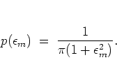$$p(\epsilon_m) \; = \; \frac{1}{\pi(1+\epsilon_m^2)}.$$ (5.50)

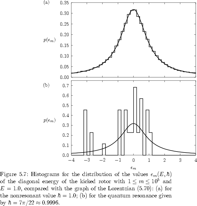
Figure 5.8a confirms this generic distribution of the $\epsilon_m$ in the case of $E=1.0$ and $\hbar =1.0$.

Figure 5.8b, on the other hand, shows the distribution of the $\epsilon_m$ for the just slightly detuned value $\hbar=7\pi/22\approx 0.9996$; in this particular example of quantum resonance, due to the implicit modulo operation in equation (5.58) $\epsilon_m$ takes on only 18 different values, as opposed to the continuous range of values obtained for $\hbar =1.0$. Thus it may be claimed that for resonant values of $\hbar$ the resulting $p(\epsilon_m)$ is not well-behaved enough (e.g. not smooth enough) for FURSTENBERG's theorem to apply. This interpretation is in agreement with the well-known fact that in the resonant case the quantum states typically (but not always) are delocalized [Fis93]. For nonresonant $\hbar$, and thus for a Lorentzian quasi-random distribution of the diagonal energies, it can be shown (see equation (B.6) in appendix B) that FURSTENBERG's integrability condition (B.2) is satisfied.

For the above reasoning the presence of the additional factor $1/W_1$ in the matrix element $\big(\cal{T}_m\big)_{11}$ of equation (5.61) (as compared with equation (5.33)) is irrelevant: the condition (B.2) is satisfied for the matrix (5.61) if and only if it is satisfied for the matrix (5.33).

Note that the quantum resonances (5.67) are an entirely quantum mechanical phenomenon that does not have a classical counterpart. In this respect the quantum resonances of the kicked rotor are similar to the quantum resonances (4.7, 4.44, 4.49) of the resonant (with respect to $T$) kicked harmonic oscillator discussed in subsections 4.1.2 and 4.2.2. The resonances (1.23/4.22) with respect to $T$, on the other hand, can also be viewed as a truly quantum mechanical phenomenon, but nevertheless they play an important role classically, too.

Putting all the above pieces together, a mapping from the quantum kicked rotor in the case of quantum nonresonance onto the ANDERSON-LLOYD model -- defined by equations (5.33, 5.34, 5.41) -- has been established, and the results on ANDERSON localization reviewed in the previous subsection carry over to the rotor. Using the same genericity assumptions as in subsection 5.1.2 (see pages f), the averaged time-independent quasienergy states $\left\vert \overline{u}_E \right>$ are found to be exponentially localized with respect to rotor (angular momentum) eigenstates; the localization length $1/\gamma$ can be derived along the same lines as equation (5.42) for $\eta=0$, $\delta=1$:

$$\cosh\gamma \; = \; \sqrt{1+\frac{1}{4W_1^2}}.$$ (5.51)

This in turn means that every generic sequence of states $\left\vert \psi_n \right>, n\in\mathbb{Z}$, generated by the quantum map (5.43) consists of localized states. In other words: the quantum kicked rotor is ANDERSON-localized. Consequences of this type of localization of quantum states are discussed below in sections 5.2 and 5.3 with respect to similarly localized states of the quantum kicked harmonic oscillator.

It is interesting to note the different roles the parameters $V_0$ and $\hbar$ play with respect to the details of the localization mechanism. Regardless of the value of $V_0$, the (resonant or nonresonant) value of $\hbar$ alone decides on the existence of localization. $V_0$, on the other hand, divided by $\hbar$ controls the localization length via equations (5.59) and (5.71).

While by the above arguments it has been shown that there exists a very close relationship between the quantum kicked rotor and the ANDERSON model, it has to be stressed that until now no mathematically rigorous proof has been found for exact equivalence of both model systems [CIS98], one of the reasons being that a tight binding equation for the rotor is obtained as an -- albeit good -- approximation only; in addition, the consequences of the quantum resonances (5.67) for such a potential proof are not yet completely understood. The ongoing effort to establish a complete analogy between the quantum kicked rotor and an ANDERSON-like model is documented in [AZ96,CIS98,AZ98], for example. The lack of mathematically rigorous equivalence may also be expressed by noting that the sample kick potential (5.64), which leads to the tight binding equation (5.66), differs from the original kick potential (5.2). Nevertheless, this explanation of localization in the quantum kicked rotor is generally accepted, and all available numerical evidence supports the equivalence of the two model systems, as far as localization is concerned [Haa01].

In this way the numerical findings of subsection 5.1.1, especially the results on saturation of energy growth of the quantum kicked rotor displayed in figure 5.4, find a satisfactory explanation.

Footnotes

... as^5.7

In general, $W_{m'}$ does not take on real values only. However, for kick potentials $V(\vartheta)$ that are even with respect to $\vartheta=\pi$, $W_{m'}$ is real, thus justifying the characterization as an energy. The potential (5.2) falls into this category.

... matrix^5.8

Without loss of generality $W_1$ can be assumed to be nonzero -- this assumption is identical with assuming nontriviality of the tight-binding equation (5.60) -- such that dividing by $W_1$ is not a problem: for the construction of the appropriate tight binding system it suffices to consider the first nonvanishing matrix element $W_{m_1'}$. A sample tight binding equation with $m_1'=2$ is given below in equation (5.101). (But note that that equation is for the kicked harmonic oscillator rather than the kicked rotor; this accounts for some differences in details which are discussed there.)

... quasi-random^5.9

In the case of quantum-nonresonance in the sense of equation (5.67), despite the deterministic quadratic dependence on $m$, $\varphi_m$ effectively becomes randomly distributed in the interval $[-\pi/2,\pi/2]$ by the implicit modulo operation, due to the periodicity of the tangent in equation (5.58).