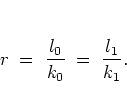
The analysis described in the previous section can be extended in order to give a qualitative explanation of the energy growth that has been observed in subsection 4.1.2 as a result of the unbounded quantum dynamics in the channels of the quantum stochastic web. In this way, contact is made with the classical counterpart not only with respect to the symmetries of the phase portrait -- thereby taking a static point of view -- but also with respect to the most important dynamical property of the system.
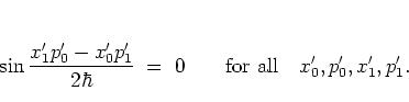
The existence of a complete set of extended states implies that,
with respect to almost all initial states
![]() ,
unbounded growth of the energy expectation value as a function of time
is to
be expected.
,
unbounded growth of the energy expectation value as a function of time
is to
be expected.
In order to check the explicit time dependence of this energy growth
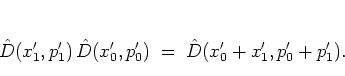
the commutation properties of different translation operators must be
considered.
Using the BCH formula
For this value of ![]() it follows from equations (4.34) and
(4.37)
that
it follows from equations (4.34) and
(4.37)
that
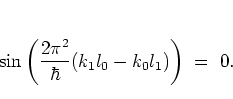
![]() is
equivalent to
is
equivalent to
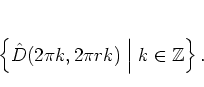
If ![]() is given by equation (4.44), then the commuting
translation operators in any case form the two-parameter group
(4.45),
regardless of equation (4.42) being satisfied
in addition or not.
is given by equation (4.44), then the commuting
translation operators in any case form the two-parameter group
(4.45),
regardless of equation (4.42) being satisfied
in addition or not.
For these two values of ![]() , commuting translation operators are
obtained
from equations (4.33) and
(4.37)
if and only if
, commuting translation operators are
obtained
from equations (4.33) and
(4.37)
if and only if
While the above shows that the cases of ![]() 4 and 6 are
essentially equivalent
with respect to commutation of translation operators,
the situation is
substantially
different for
4 and 6 are
essentially equivalent
with respect to commutation of translation operators,
the situation is
substantially
different for ![]() or
or ![]() ,
because here
,
because here ![]() and
and ![]() can take on any real value.
I do not discuss these cases any further.
can take on any real value.
I do not discuss these cases any further.
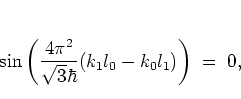
Equations (4.44) and (4.49) represent a new
kind of quantum resonance with respect to ![]() .
It has no classical counterpart and is thus entirely different from the
resonance condition (1.23/4.22)
that concerns the parameter
.
It has no classical counterpart and is thus entirely different from the
resonance condition (1.23/4.22)
that concerns the parameter ![]() and plays quite
the same
role both classically and quantum mechanically, as discussed earlier.
The consequences of the quantum resonances
(4.44, 4.49) have been studied numerically
in subsection 4.1.2.
and plays quite
the same
role both classically and quantum mechanically, as discussed earlier.
The consequences of the quantum resonances
(4.44, 4.49) have been studied numerically
in subsection 4.1.2.
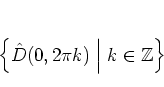
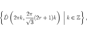
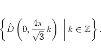
In this way, for
![]() the existence of the commutative groups
(4.41, 4.45,
4.47, 4.50)
of translation operators,
each
commuting with the
the existence of the commutative groups
(4.41, 4.45,
4.47, 4.50)
of translation operators,
each
commuting with the ![]() -th power of the FLOQUET operator,
has been established.
This is the setting of BLOCH's theorem [Mad78].
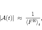
The associated energy growth can
now
be estimated qualitatively as follows.
-th power of the FLOQUET operator,
has been established.
This is the setting of BLOCH's theorem [Mad78].
The associated energy growth can
now
be estimated qualitatively as follows.
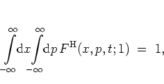
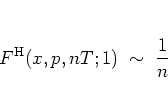
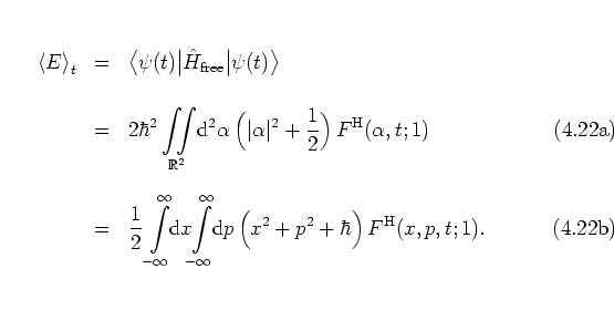
The first step is to express the energy expectation value in terms of
the HUSIMI distribution function
![]() corresponding to the state
corresponding to the state
![]() .
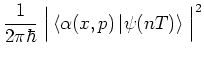
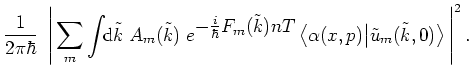
With equation (2.31) and the
overcompleteness relation (A.52) of the
coherent states I obtain for all
.
With equation (2.31) and the
overcompleteness relation (A.52) of the
coherent states I obtain for all ![]() :
:
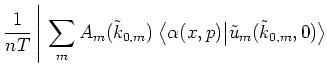
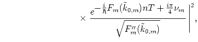
Integrals of this kind can be approximately evaluated by considering
the phase space
region
![]() significantly occupied by the
HUSIMI distribution at time
significantly occupied by the
HUSIMI distribution at time ![]() . From the normalization property
(A.53) of
. From the normalization property
(A.53) of
![]() ,
,
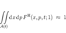 |
(4.23) |
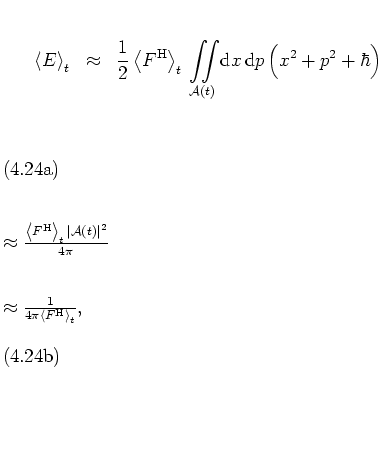
where in the intermediate step it has also been assumed that
on the average
![]() grows isotropically in the phase plane --
a behaviour that is typical for the dynamics with
grows isotropically in the phase plane --
a behaviour that is typical for the dynamics with
![]() :
cf. figures
4.2,
4.4 and
4.6
(this behaviour is in contrast to the nonisotropic growth of
:
cf. figures
4.2,
4.4 and
4.6
(this behaviour is in contrast to the nonisotropic growth of
![]() for
for ![]() , examples of which are shown in figures
C.38-C.40
in appendix C).
, examples of which are shown in figures
C.38-C.40
in appendix C).
From here on the discussion has to distinguish between the cases of
the one-parameter groups (4.41, 4.47)
and the two-parameter groups (4.45, 4.50)
of commuting translation operators.
In the first case, there exists a complete set of common eigenstates
![]() of
of ![]() and, for example,
and, for example,
![]() or
or
![]() ;
the indices
;
the indices
![]() ,
,
![]() label the eigenstates of
label the eigenstates of ![]() and
and
![]() , respectively.
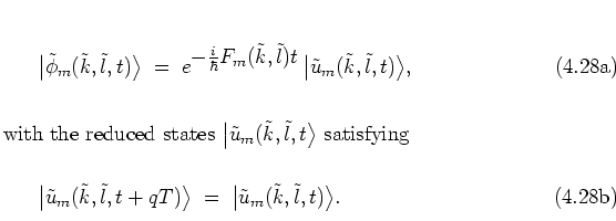
These states share the most important properties of the
quasienergy states (2.20).
In particular, they can be written as
, respectively.
These states share the most important properties of the
quasienergy states (2.20).
In particular, they can be written as
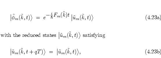
analogous to the
![]() of equation (2.23).
The phase in the exponential in the full states
(4.56a) is essentially
determined by
of equation (2.23).
The phase in the exponential in the full states
(4.56a) is essentially
determined by
![]() which parallels the
quasienergy
which parallels the
quasienergy ![]() in the states (2.20).
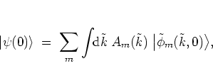
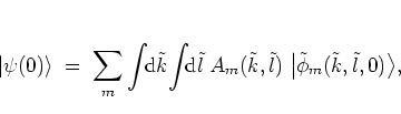
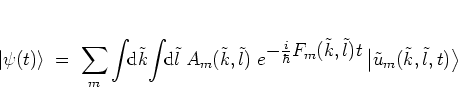
Due to the completeness of
in the states (2.20).
Due to the completeness of
![]() ,
any initial state
,
any initial state
![]() can be expanded as
can be expanded as
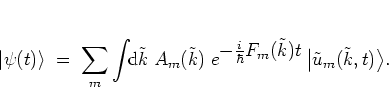 |
(4.24) |
![$F_m''(\tilde{k}_{0,m})\!\! {\protect\begin{array}{c}
<\protect\\ [-0.3cm]>
\protect\end{array}} \!0$](img857.png) .
Initial states
.
Initial states
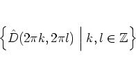
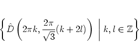
For the two-parameter groups of commuting translation operators in
the cases of the ![]() -resonances (4.44) and
(4.49),
the above reasoning can be repeated in a similar, but not identical,
fashion. The differences in some details account for a result that is
remarkably different from equation (4.62).
-resonances (4.44) and
(4.49),
the above reasoning can be repeated in a similar, but not identical,
fashion. The differences in some details account for a result that is
remarkably different from equation (4.62).
With the two-parameter groups
(4.45, 4.50),
there is a complete set of common eigenstates
![]() of
of
![]() and, for example,
and, for example,
![]() and
and
![]() (or
(or
![]() and
and
![]() );
corresponding to the two group parameters there are now two indices
);
corresponding to the two group parameters there are now two indices
![]() in addition to
in addition to ![]() .
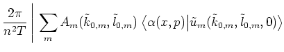
Parallel to equations (4.56) I now have
.
Parallel to equations (4.56) I now have
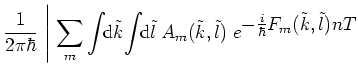
The initial state
 |
(4.29) |
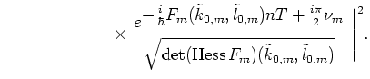
 |
|||
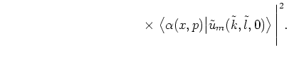 |
(4.30) |
The above explanation for the energy growth relies on the possibility to expand the states as in equations (4.57) and (4.64), and on the applicability of the stationary phase approximation. In particular the expansions (4.57, 4.64) are somewhat questionable; their -- at least approximate -- validity depends on details of the spectral properties of the respective operators. Nevertheless, the arguments based on these assumptions yield suggestive results, in accordance with the numerical findings in section 4.1.2. These points are discussed in some more detail in [GB93,BR95].
This
chapter provides a description of the
typical
quantum dynamics
of the kicked harmonic oscillator in the cases of resonance with
![]() .
It is
natural to ask in which way the quantum dynamics in the
complementary cases of nonresonance
-- where there are no phase space structures characterized by
combined translational and rotational symmetries
--
differs from the scenario of the present chapter.
It might be conjectured
that in the absence of resonance, without the condition
(1.23/4.22) enforcing the
existence of infinitely extended quantum states,
the typical quantum dynamics
is characterized by some kind of
localization phenomenon.
That
conjecture can be considered to be motivated by
the multitude of localization results
that have been obtained for the quantum kicked rotor,
for which the absence of a classical resonance condition like
(1.23) is an essential feature.
This question is addressed in the following chapter
5, where the localization approach to the
dynamics is taken.
.
It is
natural to ask in which way the quantum dynamics in the
complementary cases of nonresonance
-- where there are no phase space structures characterized by
combined translational and rotational symmetries
--
differs from the scenario of the present chapter.
It might be conjectured
that in the absence of resonance, without the condition
(1.23/4.22) enforcing the
existence of infinitely extended quantum states,
the typical quantum dynamics
is characterized by some kind of
localization phenomenon.
That
conjecture can be considered to be motivated by
the multitude of localization results
that have been obtained for the quantum kicked rotor,
for which the absence of a classical resonance condition like
(1.23) is an essential feature.
This question is addressed in the following chapter
5, where the localization approach to the
dynamics is taken.
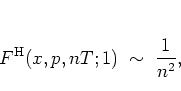
These observations,
together with the fact that
the conclusions obtained on the basis of the
assumptions leading to the
approximation (4.55a)
obviously agree with the numerical results of section
4.1.2
(this is discussed on pages
![[*]](crossref.png) ff
below),
further explain the importance of the HUSIMI distribution for the analysis of the quantum dynamics of classically
chaotic systems.
ff
below),
further explain the importance of the HUSIMI distribution for the analysis of the quantum dynamics of classically
chaotic systems.
![\begin{displaymath}
e^{\textstyle {\hat{A}}} e^{\textstyle {\hat{B}}} \; = \; e...
...{\hat{B}}} \; e^{\textstyle \frac{1}{2}[{\hat{A}},{\hat{B}}]},
\end{displaymath}](img797.png)
![\begin{displaymath}
\left[ {\hat{D}}(x_1',p_1'),{\hat{D}}(x_0',p_0') \right]
\...
..._1'p_0'-x_0'p_1'}{2\hbar} \,
{\hat{D}}(x_0'+x_1',p_0'+p_1') .
\end{displaymath}](img799.png)