As discussed in the previous subsection,
both
discrete SCHRÖDINGER equations (5.94a, 5.94b)
in a natural way
give rise
to the
approximating tight-binding equation
In terms of the transfer matrix formalism of subsection
5.1.2, the definitions
However, this formulation is disadvantageous for several reasons.
First, it rests on the assumption that
![]() for all
for all ![]() ,
because
,
because ![]() makes up the denominators of two of
the matrix elements of the transfer matrix (5.102).
Unfortunately, this assumption cannot be checked
analytically for
all combinations
of
makes up the denominators of two of
the matrix elements of the transfer matrix (5.102).
Unfortunately, this assumption cannot be checked
analytically for
all combinations
of ![]() and
and ![]() ,
because
a closed solution of the integral in equation (5.86)
is
not
available.
Already a single
,
because
a closed solution of the integral in equation (5.86)
is
not
available.
Already a single
![]() with
with
![]() could spoil the whole
theory.
Even more,
could spoil the whole
theory.
Even more,
The workaround
for the case of a vanishing (second-) nearest neighbour matrix element
sketched in
the footnote
on page ![[*]](crossref.png) only works
in the context of the kicked rotor,
because of the translation invariance of the discrete
SCHRÖDINGER equation
for that model.
This is
in contrast to
the translation
noninvariance
of the discrete SCHRÖDINGER equation
of the kicked harmonic oscillator, i.e.
the explicit
only works
in the context of the kicked rotor,
because of the translation invariance of the discrete
SCHRÖDINGER equation
for that model.
This is
in contrast to
the translation
noninvariance
of the discrete SCHRÖDINGER equation
of the kicked harmonic oscillator, i.e.
the explicit
![]() -dependence of the oscillator's hopping matrix element
-dependence of the oscillator's hopping matrix element ![]() for
the interaction with the nearest neighbour at the
for
the interaction with the nearest neighbour at the ![]() -th site.
Divisions by
-th site.
Divisions by ![]() occur in all transfer matrix models of
the kicked harmonic oscillator, including those to be discussed below,
and, as a matter of principle, cannot be avoided.
In which sense
the condition (5.105)
can be taken to be satisfied is addressed in some more detail in
subsection 5.3.4.
occur in all transfer matrix models of
the kicked harmonic oscillator, including those to be discussed below,
and, as a matter of principle, cannot be avoided.
In which sense
the condition (5.105)
can be taken to be satisfied is addressed in some more detail in
subsection 5.3.4.
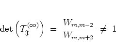
A second, and more important, disadvantage is that the transfer matrices
of equation (5.102)
do not satisfy the unimodularity requirement of FURSTENBERG's theorem:
 |
(5.78) |
Finally, backpropagation
towards the left
cannot simply be accomplished as in the case of the rotor
by using the same transfer matrices
![]() as for propagation to the right
and setting
as for propagation to the right
and setting
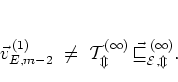
In the light of these shortcomings of the model specified by the matrix (5.102), the question needs to be addressed if and how the localization results of subsection 5.1.2 carry over to the oscillator.
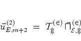
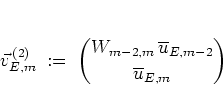
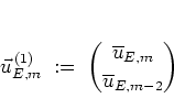
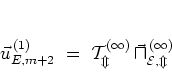
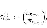
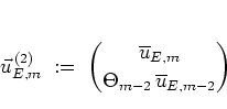
One way to approach this problem
is to define the
more general vectors
Equations (5.113,
5.114)
and the dynamical equation
For proving localization in the kicked harmonic oscillator it suffices
to consider the transfer dynamics in positive ![]() -direction,
because the
lattice on which the discrete SCHRÖDINGER equation of the oscillator
is defined is
infinite towards the right only,
as opposed to the bi-infinite lattice in the case of the rotor.
So localization towards the left is automatically built into the system
by the condition
-direction,
because the
lattice on which the discrete SCHRÖDINGER equation of the oscillator
is defined is
infinite towards the right only,
as opposed to the bi-infinite lattice in the case of the rotor.
So localization towards the left is automatically built into the system
by the condition ![]() ,
once FURSTENBERG's theorem has been shown
to apply.
Nevertheless it is instructive to establish the analogy with the
conventional tight binding models as far-reaching as possible.
In fact, using the models discussed below, exponential localization is
typically found
in both directions
-- cf. figures 5.12a,
5.12b.
What is more, a discrete point spectrum of energy eigenvalues
describing the localized dynamics
can only be expected in the case of exponential localization in both
directions -- cf. subsection 5.1.2.
,
once FURSTENBERG's theorem has been shown
to apply.
Nevertheless it is instructive to establish the analogy with the
conventional tight binding models as far-reaching as possible.
In fact, using the models discussed below, exponential localization is
typically found
in both directions
-- cf. figures 5.12a,
5.12b.
What is more, a discrete point spectrum of energy eigenvalues
describing the localized dynamics
can only be expected in the case of exponential localization in both
directions -- cf. subsection 5.1.2.
In the rotor case,
the same transfer matrix can be used for right- and leftward
dynamics on the lattice, provided the two different sets of vectors
![]() ,
, ![]() of equations (5.62)
are used.
For the oscillator, on the other hand, the nontriviality of the
off-diagonal matrix elements of the
of equations (5.62)
are used.
For the oscillator, on the other hand, the nontriviality of the
off-diagonal matrix elements of the
![]() necessitates the
introduction of
another set of
transfer matrices for leftward transfer.
No vectors
necessitates the
introduction of
another set of
transfer matrices for leftward transfer.
No vectors
![]() ,
,
![]() could be
constructed that allow to model the
tight binding equation (5.101)
using the same matrix for
propagation into both directions.
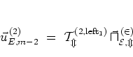
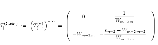
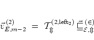
In a sense,
the situation in the oscillator case is reversed, as compared to the
rotor: the simplest formulation of backpropagation is
obtained by
using the same vectors
could be
constructed that allow to model the
tight binding equation (5.101)
using the same matrix for
propagation into both directions.
In a sense,
the situation in the oscillator case is reversed, as compared to the
rotor: the simplest formulation of backpropagation is
obtained by
using the same vectors
![]() as for propagation in positive
as for propagation in positive ![]() -direction, but
another set of
transfer matrices, namely
(quite naturally)
the inverses of the
-direction, but
another set of
transfer matrices, namely
(quite naturally)
the inverses of the
![]() :
:
The above construction of a tight-binding model for the kicked harmonic
oscillator is made to be as close to the corresponding model for the
kicked rotor as possible. However, comparing equations
(5.114,
5.117,
5.120)
with their rotor counterpart (5.61) makes it clear
that the harmonic oscillator case is considerably more intricate,
due to the presence of ![]() and
and ![]() in the matrix elements.
This makes the application of FURSTENBERG's theorem more
difficult than in the canonical rotor case.
in the matrix elements.
This makes the application of FURSTENBERG's theorem more
difficult than in the canonical rotor case.
In many cases,
the transfer matrices ![]() defined in equations
(5.114, 5.117, 5.120)
satisfy the
assumptions
of FURSTENBERG's theorem:
the
defined in equations
(5.114, 5.117, 5.120)
satisfy the
assumptions
of FURSTENBERG's theorem:
the ![]() are all unimodular by construction,
the
respective
groups generated by the sets
are all unimodular by construction,
the
respective
groups generated by the sets
![]() are noncompact and irreducible in the sense of
appendix B, and all available numerical evidence
supports the assumption that the
are noncompact and irreducible in the sense of
appendix B, and all available numerical evidence
supports the assumption that the ![]() considered
give rise to ``sufficiently
well-behaved'' measures
considered
give rise to ``sufficiently
well-behaved'' measures ![]() as defined by the
integrability
condition (B.2).
as defined by the
integrability
condition (B.2).
The last remark may be made more explicit by
discussing
in some more detail
the assumptions of FURSTENBERG's theorem
for the ![]() considered here.
From appendix B,
the integrability condition is
considered here.
From appendix B,
the integrability condition is
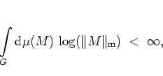
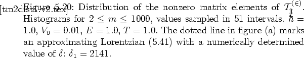
In order to establish the validity of the condition
(B.2) with
respect to the maximum norm, the distributions of values of the matrix
elements of the ![]() need to be checked.
The off-diagonal matrix elements of
need to be checked.
The off-diagonal matrix elements of
![]() ,
,
![]() and
and
![]() are determined
by the nearest neighbour interactions
are determined
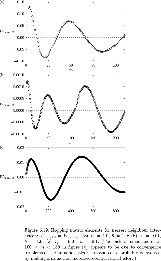
by the nearest neighbour interactions ![]() , for which no closed
formula is available, as discussed earlier. Nevertheless, the
corresponding distribution of values can be studied numerically.
Figures 5.21b, 5.21c
and
, for which no closed
formula is available, as discussed earlier. Nevertheless, the
corresponding distribution of values can be studied numerically.
Figures 5.21b, 5.21c
and
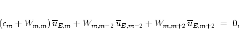
It remains to
investigate
the nontrivial diagonal matrix elements of the ![]() ,
namely
,
namely
Summarizing, although
a rigorous
proof is lacking, there is good reason
-- including some convincing numerical evidence --
to assume that
typically
the condition
(B.2) is satisfied for the matrices
![]() ,
,
![]() and
and
![]() modelling the
kicked harmonic oscillator.
modelling the
kicked harmonic oscillator.
As a result,
I have shown that
at least for some combinations of values of the parameters,
FURSTENBERG's theorem can be applied to the transfer matrix
formulation
of the kicked harmonic oscillator in
a way which is largely analogous to the conventional procedure
in the case of the kicked rotor;
it may be assumed that similar results probably hold for many other
values of the parameters.
By the same reasoning as in subsection 5.1.3 it
can be concluded that
the norms of the vectors
![]() and
and
![]() generated by the respective equations of motion decay exponentially, which
in turn implies the same for the absolute values of the expansion
coefficients
generated by the respective equations of motion decay exponentially, which
in turn implies the same for the absolute values of the expansion
coefficients
![]() of the quasienergy states discussed
in subsection 5.3.1.
This finally establishes the result that the nonresonant kicked harmonic
oscillator exhibits ANDERSON localization, provided the
parameters are such that the conditions are met which I have discussed
above.
When this is the case then generic sequences of states
of the quasienergy states discussed
in subsection 5.3.1.
This finally establishes the result that the nonresonant kicked harmonic
oscillator exhibits ANDERSON localization, provided the
parameters are such that the conditions are met which I have discussed
above.
When this is the case then generic sequences of states
![]() generated by the quantum map
(5.72) consist of exponentially localized
states.
The states are localized with respect to
the basis of
harmonic oscillator eigenstates,
and therefore they are localized in phase space
as well.
Figure 5.12
stresses
the first aspect of localization;
figures
5.9 through
5.11
and the examples in section C.4 of
the appendix
demonstrate localization in phase space.
generated by the quantum map
(5.72) consist of exponentially localized
states.
The states are localized with respect to
the basis of
harmonic oscillator eigenstates,
and therefore they are localized in phase space
as well.
Figure 5.12
stresses
the first aspect of localization;
figures
5.9 through
5.11
and the examples in section C.4 of
the appendix
demonstrate localization in phase space.
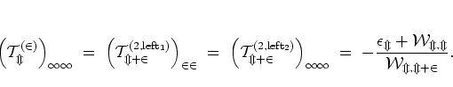
As discussed in subsection 5.1.2, a lower bound for
the speed of the decay of
![]() is established via the
LIAPUNOV exponent of the corresponding transfer matrices. From this
point of view it
does not come as a surprise
that in the case of the oscillator the transfer matrices
is established via the
LIAPUNOV exponent of the corresponding transfer matrices. From this
point of view it
does not come as a surprise
that in the case of the oscillator the transfer matrices
![]() and
and
![]() or
or
![]() do not coincide as they do in the case of the rotor.
This is again a consequence of the asymmetry expressed by the inequality
(5.87) and can lead to different speeds of convergence to
zero of
do not coincide as they do in the case of the rotor.
This is again a consequence of the asymmetry expressed by the inequality
(5.87) and can lead to different speeds of convergence to
zero of
![]() on the right and on the left.
But note that FURSTENBERG's theorem provides a lower bound on the speed
of convergence only; the speed may be actually larger, and
in special cases
it
can
coincide on the right and on the left.
on the right and on the left.
But note that FURSTENBERG's theorem provides a lower bound on the speed
of convergence only; the speed may be actually larger, and
in special cases
it
can
coincide on the right and on the left.
Inevitably, the
above discussion of the distribution of values of the matrix elements
-- especially of the off-diagonal matrix elements --
of the transfer matrices
is to some degree heuristic,
and therefore the same is true, unfortunately, with
respect to the distribution ![]() of the transfer matrices.
In particular the arguments in favour of nicely distributed off-diagonal
matrix elements leading to FURSTENBERG-integrability are
but qualitative.
This problem is addressed -- and solved -- in
subsection 5.3.3 by considering a
different class of transfer matrices.
of the transfer matrices.
In particular the arguments in favour of nicely distributed off-diagonal
matrix elements leading to FURSTENBERG-integrability are
but qualitative.
This problem is addressed -- and solved -- in
subsection 5.3.3 by considering a
different class of transfer matrices.
![\begin{displaymath}
\cal{T}_m^{(1)}
\; := \; \left( \begin{array}{cc}
\displa...
...W_{m,m-2}} {W_{m,m+2}} \\ [0.6cm]
1 &
0
\end{array} \right)
\end{displaymath}](img1165.png)
![\begin{displaymath}
\cal{T}_m^{(2)}
\; := \; \left( \begin{array}{cc}
\displa...
...ac{1}{\Theta_m} \\ [0.6cm]
\Theta_m &
0
\end{array} \right)
\end{displaymath}](img1185.png)
![\begin{displaymath}
\cal{T}_m^{(2)}
\; = \; \left( \begin{array}{cc}
\display...
...1}{W_{m,m+2}} \\ [0.6cm]
W_{m,m+2} &
0
\end{array} \right).
\end{displaymath}](img1195.png)