In the previous subsection implicitly the ``classical'' approach to the
modelling by means of transfer matrices was
followed:
only the first
component of the vector equations
(5.115, 5.116, 5.119)
was constructed to be equivalent to the tight binding equation
(5.101), while the second component
was made to be a trivial identity by construction;
in addition, only the three amplitudes
![]() ,
,
![]() and
and
![]() were allowed to contribute for any given
were allowed to contribute for any given ![]() .
In the present
subsection I use a
more general
starting point for deriving transfer matrices
which are
more suitable for proving localization than
.
In the present
subsection I use a
more general
starting point for deriving transfer matrices
which are
more suitable for proving localization than
![]() ,
,
![]() and
and
![]() .
.
Generalized or higher order transfer matrix models reformulating
the tight binding equation (5.101) can be
introduced
by considering ![]() -dimensional transfer matrices
(rather than the only two-dimensional transfer matrices as used up to this
point) with some suitable
-dimensional transfer matrices
(rather than the only two-dimensional transfer matrices as used up to this
point) with some suitable ![]() :
:
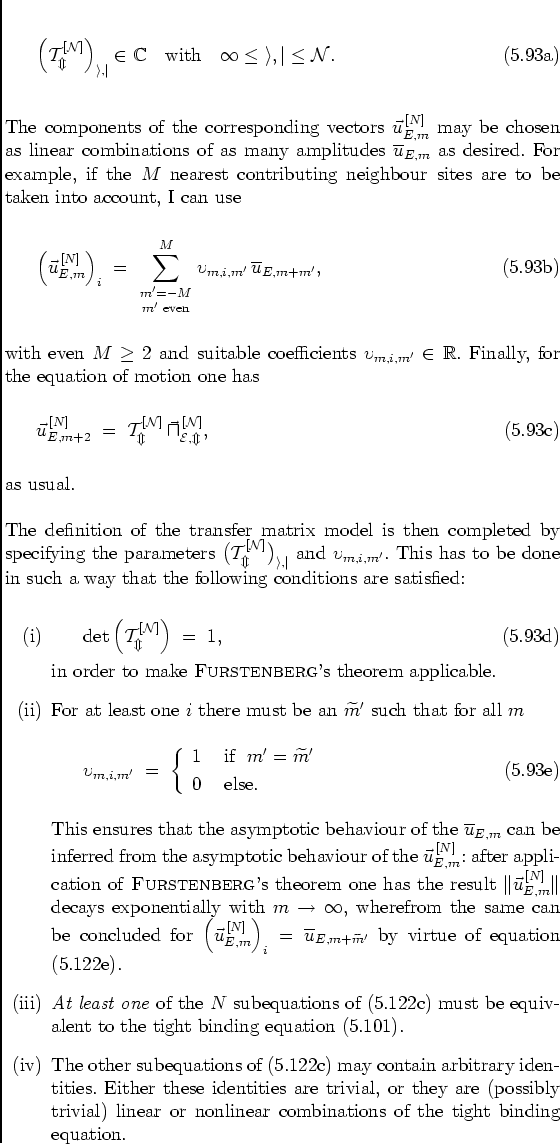
The importance of condition (iii) is easily underestimated.
It avoids the construction of models that are only consistent with
the tight binding equation, without being equivalent to it. Such a
situation occurs, for example, if one specifies the parameters in such a
way that
the only nontrivial subequation of (5.122c) is a
nontrivial
linear combination of
(5.101);
then it is not guaranteed that the
solutions
![]() of such a model also satisfy the tight
binding equation.
of such a model also satisfy the tight
binding equation.
This scheme allows to construct a multitude of different transfer matrix models. Once a model has been defined in this way, the remaining conditions of FURSTENBERG's theorem need to be checked, thus possibly leading to a proof of localization, if the model has been constructed properly.
Following this scheme, one can discuss the transfer matrix model with
![]() and
and ![]() , for example.
I have tried to choose the 18
parameters of this model in such a way that the resulting expressions
are as simple as possible. After some
(lengthy)
algebra, the
transfer matrix
, for example.
I have tried to choose the 18
parameters of this model in such a way that the resulting expressions
are as simple as possible. After some
(lengthy)
algebra, the
transfer matrix
The
system (5.123) is suited for
propagation in positive ![]() -direction.
Backpropagation can be achieved by using
-direction.
Backpropagation can be achieved by using
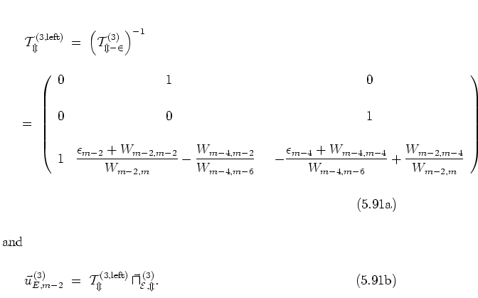
It is easy to see -- by explicitly writing down all three subequations -- that the first subequation of the equation of motion (5.123c) contains the tight binding equation three times (in the sense of (iv)), the second subequation is equivalent to the tight-binding equation (satisfying condition (iii)), and the third subequation is just a trivial identity.
The
![]() do not share the
worst
disadvantage of the
do not share the
worst
disadvantage of the
![]() discussed in the previous subsection.
Most matrix elements take on the trivial values 0 or 1,
which are uncritical with respect to the integrability condition
(B.2);
the only
nontrivial matrix elements,
discussed in the previous subsection.
Most matrix elements take on the trivial values 0 or 1,
which are uncritical with respect to the integrability condition
(B.2);
the only
nontrivial matrix elements,
![]() and
and
![]() ,
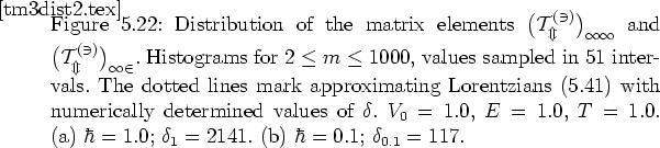
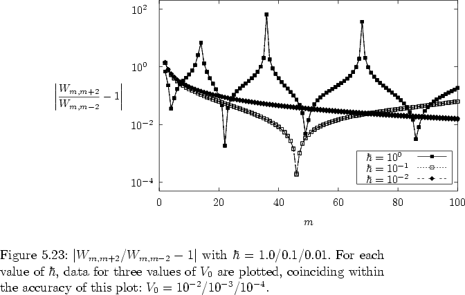
are characterized by Lorentzian distributions of values, as
figure 5.23 shows.
,
are characterized by Lorentzian distributions of values, as
figure 5.23 shows.
Summarizing, for the parameters considered explicitly, and most probably
for all parameter combinations belonging to the nonpathological
systems with
![]() for all
for all ![]() ,
,
![]() and
and
![]() satisfy
the integrability condition (B.2)
and therefore give rise to
quantum localization of the
satisfy
the integrability condition (B.2)
and therefore give rise to
quantum localization of the ![]() -nonresonant kicked harmonic oscillator;
the localization mechanism is identified as that of classical
ANDERSON localization.
-nonresonant kicked harmonic oscillator;
the localization mechanism is identified as that of classical
ANDERSON localization.