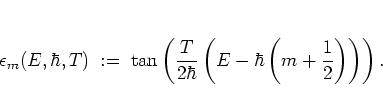
Although classically the kicked rotor (5.1) and the kicked harmonic oscillator (1.17) are fundamentally different, for example in that the kicked rotor is characterized by one frequency only (namely the frequency of the kick) whereas the kicked oscillator has two frequencies (the second being the frequency of the unperturbed harmonic dynamics), the quantum localization phenomena in both models can be explained by the same mechanism. This mechanism is described by the theory of ANDERSON localization as outlined in section 5.1. I now show that this theory -- with some alterations due to the differing eigenstates of the two model systems -- can also be applied to the quantum kicked harmonic oscillator.
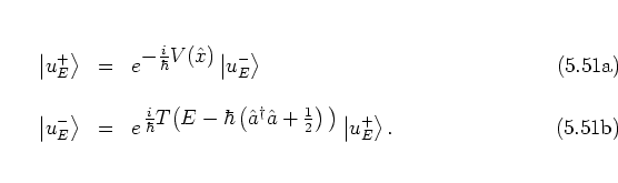
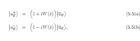
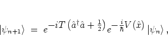
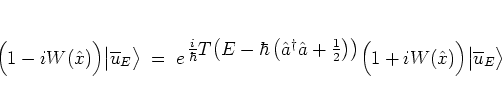
As in equation (5.43) I begin with the quantum
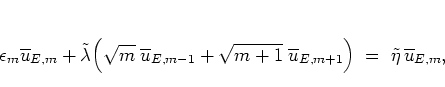
map (2.37) for the kicked harmonic oscillator,
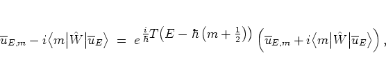
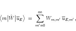
Projecting equation (5.77) onto the eigenstates
![]() of the free harmonic oscillator (cf. equation (2.38)), I get
of the free harmonic oscillator (cf. equation (2.38)), I get
 |
(5.52) |
 |
(5.56) |
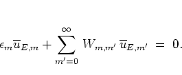
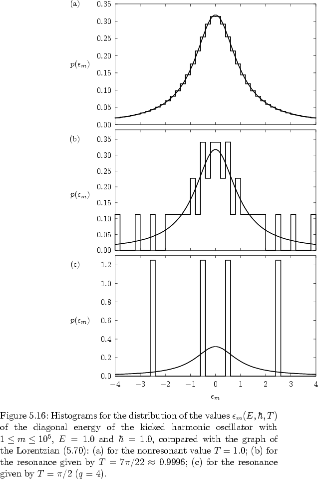
The first remark concerns the diagonal energies.
As their rotor counterparts,
the
![]() can be viewed as being generated by a
(quasi-)
random
number generator that follows a Lorentzian distribution
(5.70),
provided a
condition of nonresonance is satisfied. Because of the different
expressions (5.58) and (5.81)
defining the respective diagonal energies, the (non-) resonances in
question differ, too. For the quantum kicked oscillator, the
quantum resonances
inhibiting quasi-randomness of the
can be viewed as being generated by a
(quasi-)
random
number generator that follows a Lorentzian distribution
(5.70),
provided a
condition of nonresonance is satisfied. Because of the different
expressions (5.58) and (5.81)
defining the respective diagonal energies, the (non-) resonances in
question differ, too. For the quantum kicked oscillator, the
quantum resonances
inhibiting quasi-randomness of the ![]() are given by
are given by
The
fact that the
resonance condition
(1.22/4.21a)
-- and thereby the important special case
(1.23/4.22) as well --,
which is essential for the formation of classical and
quantum stochastic webs, naturally arises
as equation (5.85) in this quantum
theory and characterizes those situations where no quantum localization
can be expected, is a strong argument in favour of this formulation of the
theory of localization in the kicked harmonic oscillator: in this way
proper quantum-classical correspondence is automatically
guaranteed.
What is more, in this way also the quantum theories for the cases of
resonance
and nonresonance nicely fit together in a complementary fashion.
The resonances with respect to ![]() are true quantum resonances in
the sense that they are obtained here as a consequence of a genuinely
quantum mechanical theory.
On the other hand, as discussed above, these
resonances play an important role classically as well, such that the
term ``quantum resonance'' might be questioned.
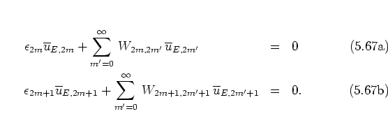
This situation is to be compared with the quantum resonances
(5.67) of the kicked rotor
and (4.7, 4.44, 4.49)
of the resonant kicked harmonic oscillator
which have no classical counterpart.
are true quantum resonances in
the sense that they are obtained here as a consequence of a genuinely
quantum mechanical theory.
On the other hand, as discussed above, these
resonances play an important role classically as well, such that the
term ``quantum resonance'' might be questioned.
This situation is to be compared with the quantum resonances
(5.67) of the kicked rotor
and (4.7, 4.44, 4.49)
of the resonant kicked harmonic oscillator
which have no classical counterpart.
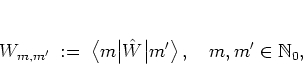
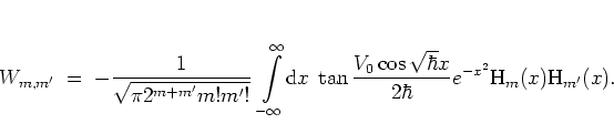
The second important difference to the case of the rotor is that
for
the oscillator the evaluation of the
hopping matrix elements
is not as simple as in
subsection 5.1.3,
since the oscillator eigenfunctions
![]() (2.39) are algebraically much more
complicated than the simple exponentials of the rotor eigenfunctions
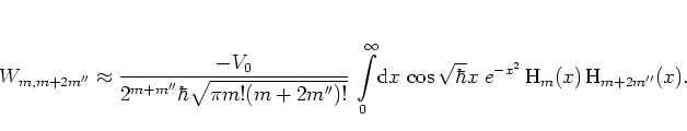
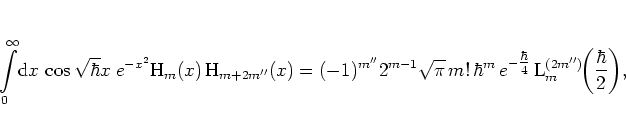
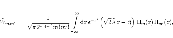
(5.12). Explicitly, the matrix elements
(5.83)
for the cosine kick potential (1.18) are given
by5.10
(2.39) are algebraically much more
complicated than the simple exponentials of the rotor eigenfunctions
(5.12). Explicitly, the matrix elements
(5.83)
for the cosine kick potential (1.18) are given
by5.10
It is obvious that, because of
the dependence on the
HERMITE polynomials, the formula (5.86) cannot be
simplified to yield an expression that depends on a single index
only
as the
corresponding rotor
matrix element (5.54):
the matrix elements ![]() have to be viewed as
functions of both the position
have to be viewed as
functions of both the position ![]() and the difference
and the difference ![]() .
This means that the interaction between the sites of the
ANDERSON lattice for the oscillator is not translation invariant;
in other words, the strength of the interaction between two sites does
not depend on their distance on the lattice
alone.
For the proof of ANDERSON localization this is not an obstacle, as long
as for all
.
This means that the interaction between the sites of the
ANDERSON lattice for the oscillator is not translation invariant;
in other words, the strength of the interaction between two sites does
not depend on their distance on the lattice
alone.
For the proof of ANDERSON localization this is not an obstacle, as long
as for all ![]() the absolute values
the absolute values ![]() of the matrix elements
decay rapidly enough with the distance
of the matrix elements
decay rapidly enough with the distance ![]() from the site
from the site ![]() ,
in much the same way as the absolute values of the rotor matrix elements
do.
,
in much the same way as the absolute values of the rotor matrix elements
do.
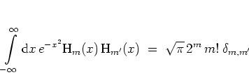
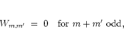
Analytically not much can be said in general about the values ![]() takes on. The only straightforward property to notice is that every
second of them vanishes,
takes on. The only straightforward property to notice is that every
second of them vanishes,
| (5.63) |
| (5.64) |
 |
(5.65) |
 |
(5.66) |
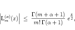
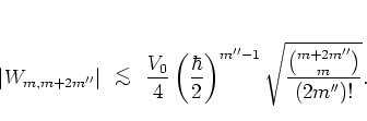
The convergence
![]() for larger values of
for larger values of ![]() is checked in figures 5.18 and
5.19;
since
the integral in equation (5.86) cannot be solved
analytically in general, the matrix elements are evaluated numerically and
plotted for several parameter combinations.
Due to the oscillatory integrand, it is difficult to obtain exact results
by numerical computation for some of these parameter combinations.
This difficulty has an
impact especially on the results for larger values of
is checked in figures 5.18 and
5.19;
since
the integral in equation (5.86) cannot be solved
analytically in general, the matrix elements are evaluated numerically and
plotted for several parameter combinations.
Due to the oscillatory integrand, it is difficult to obtain exact results
by numerical computation for some of these parameter combinations.
This difficulty has an
impact especially on the results for larger values of ![]() and becomes
worse in the case of small values of
and becomes
worse in the case of small values of ![]() , as can be seen in the
figures:
the data for
, as can be seen in the
figures:
the data for ![]() and
and ![]() in figures
5.18c and 5.19c are
spoiled by numerical round-off errors,
and the same
appears to be
true for the points with
in figures
5.18c and 5.19c are
spoiled by numerical round-off errors,
and the same
appears to be
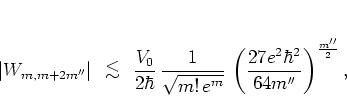
true for the points with
![$\vert m''\vert {\protect\begin{array}{c}
>\protect\\ [-0.3cm]\sim
\protect\end{array}} 10$](img1147.png) and
and ![]() or
or ![]() in figure
5.19a.
In the opposite case of small
in figure
5.19a.
In the opposite case of small ![]() and large
and large ![]() the numerical results nicely agree with the convergence to zero as
predicted by
the relation (5.93).
the numerical results nicely agree with the convergence to zero as
predicted by
the relation (5.93).
Apart from
the
numerical problems, the figures give a clear indication
of the typical behaviour of the matrix elements. The
![]() are
peaked around
are
peaked around ![]() and decay
more or less
exponentially on both sides.
Figure 5.19 also
illustrates
that in general
for any site
and decay
more or less
exponentially on both sides.
Figure 5.19 also
illustrates
that in general
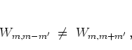
for any site ![]() the speed of this decay is not the same
for
the speed of this decay is not the same
for ![]() and
and ![]() ,
in agreement with the inequality (5.87). By taking
suitable limits
(with respect to the parameters), the
,
in agreement with the inequality (5.87). By taking
suitable limits
(with respect to the parameters), the
![]() decay fast enough to allow equation
(5.84) to approach a tight binding
equation.
Some aspects
of the case of those parameter combinations which do not give
rise to tight binding are addressed in
subsection 5.3.4 below.
decay fast enough to allow equation
(5.84) to approach a tight binding
equation.
Some aspects
of the case of those parameter combinations which do not give
rise to tight binding are addressed in
subsection 5.3.4 below.
This leads to another observation which marks a noteworthy difference to
the rotor. Above, I have discussed which conditions have to be met for
equation (5.84) to become
a tight binding equation.
Strictly speaking, equation
(5.84) with the cosine kick potential
cannot become a tight binding equation under any circumstances, because
equation (5.88) indicates that no site is coupled
to its nearest neighbour, and the closest interacting sites are
characterized by indices ![]() ,
, ![]() with
with ![]() .
Even more, the dynamics
on the sites with even indices and on the sites with odd indices
are
completely decoupled.
This means that the cosine-kicked oscillator
must
be described not by
a single,
but by a pair of discrete SCHRÖDINGER equations which are
interwoven with
but independent of
each other:
.
Even more, the dynamics
on the sites with even indices and on the sites with odd indices
are
completely decoupled.
This means that the cosine-kicked oscillator
must
be described not by
a single,
but by a pair of discrete SCHRÖDINGER equations which are
interwoven with
but independent of
each other:
In
each of these two subsystems tight binding is possible
within the approximations discussed above.
Of course, if one has tight binding in both subsystems at the same
time, then the entire system is tightly bound and prone to localization.
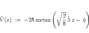
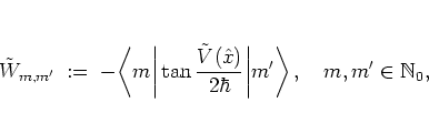
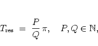
On the other hand, by choosing a different kick potential
as a replacement for the cosine potential (1.18),
 |
(5.69) |
 |
(5.70) |
![\begin{displaymath}
\tilde{W}_{m,m'}
\; = \; \left\{
\begin{array}{ccl}
\sqr...
...'=m+1 \\ [0.2cm]
0 & \: \mbox{else} \, .
\end{array} \right.
\end{displaymath}](img1161.png) |
(5.71) |
The alternate kick potential (5.95)
is intended here for nothing more than
demonstrating how a tight binding system describing the
quantum kicked harmonic oscillator can be constructed;
in particular I do not discuss the classical dynamics of the
harmonic oscillator with this kick potential here.
However, motivated by the results described in [Jun95],
one might speculate about
the existence of classical
-- and perhaps quantum mechanical? --
stochastic webs even for this aperiodic
kick potential (in cases of resonance with respect to ![]() ).
In the following I do not discuss the alternate system specified by the
potential (5.95) any further.
).
In the following I do not discuss the alternate system specified by the
potential (5.95) any further.
In this subsection I have shown that the quantum kicked harmonic oscillator can be modelled by a discrete SCHRÖDINGER equation which is similar to the model used in ANDERSON's theory. Provided certain conditions are met, it is also possible to obtain an approximative tight binding model as in the case of the rotor. In the following two subsections I discuss how these findings can be used to prove ANDERSON localization in the oscillator.
![\begin{figure}
% latex2html id marker 23017
\vspace*{-0.5cm}
\par
\hspace*{-2.0...
...W_{m,m'}=0$\ for $m+m'$\ odd. % \\
\rule[-1.0cm]{0.0cm}{1.1cm}
}
\end{figure}](img1148.png)
![\begin{figure}
% latex2html id marker 23510
\vspace*{-0.5cm}
\par
\hspace*{-2.0...
...ut for
$m=50$.
% (a)~$\hbar=1.0$;
\rule[-1.5cm]{0.0cm}{1.6cm}
}
\end{figure}](img1149.png)