Next: Discrete Dynamics
Up: The Kicked Harmonic Oscillator
Previous: Newtonian Equations of Motion
Contents
Canonical Formulation
In principle, the Newtonian equation of motion
(1.7) allows a complete
analysis of the
classical dynamics of the
kicked harmonic
oscillator. Nevertheless, it
is advantageous to use the
Hamiltonian formulation of the problem instead,
because
many classical results can be derived in this formulation with much more
ease (cf. section 1.2).
What is more,
for the discussion of the corresponding
quantum
problem
the Hamiltonian operator is
indispensable
anyway.
The dynamics of a charged particle in an electromagnetic field can be
described
by
the Hamiltonian [Gol80]
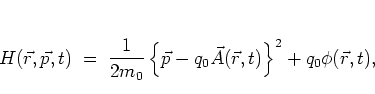 |
(1.5) |
with the momentum
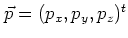 of the particle
and
the vector potential
of the particle
and
the vector potential  and the scalar potential
  for the
electromagnetic field.
The potentials
have to be chosen in such a way that the magnetic and electric fields
are obtained via
for the
electromagnetic field.
The potentials
have to be chosen in such a way that the magnetic and electric fields
are obtained via
 and
and
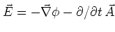 .
For the fields of equation (1.1), this is
achieved, for example, by
choosing
.
For the fields of equation (1.1), this is
achieved, for example, by
choosing
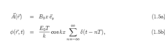
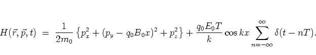
such that the corresponding Hamiltonian becomes
 is cyclic in
  and
and  . As in the previous subsection it is clear
that the dynamics in -direction is that of a free particle and
separates from the rest of the dynamics; therefore in the following
I drop the -dynamics altogether.
Cyclicity of in means that
. As in the previous subsection it is clear
that the dynamics in -direction is that of a free particle and
separates from the rest of the dynamics; therefore in the following
I drop the -dynamics altogether.
Cyclicity of in means that  is a constant of motion.
Since this constant enters the Hamiltonian
via the term
is a constant of motion.
Since this constant enters the Hamiltonian
via the term  only,
changing the value of just results in a shift of the
origin of the
only,
changing the value of just results in a shift of the
origin of the  -axis (cf. with the constant in equation
(1.6)).
Hence can be set to zero without loss of generality.
The
remaining
``essential'' part of the Hamiltonian is
-axis (cf. with the constant in equation
(1.6)).
Hence can be set to zero without loss of generality.
The
remaining
``essential'' part of the Hamiltonian is
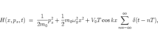 |
(1.6) |
with the parameter
 |
(1.7) |
which
controls the
amplitude
of the kick;  has the dimension of an energy.
As from here on only the momentum
has the dimension of an energy.
As from here on only the momentum  , conjugate to , is of importance
and no confusion with other momenta
can arise,
I now
drop the index .
, conjugate to , is of importance
and no confusion with other momenta
can arise,
I now
drop the index .
Naturally, the two canonical equations that follow from equation
(1.12),
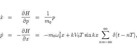 |
(1.8) |
can be combined to obtain once again the Newtonian equation of motion
(1.7).
In order to minimize the number of parameters of the system I introduce
dimensionless
variables
by the
scaling transformation
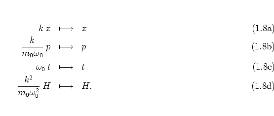
Similarly, the parameters ,  are replaced with dimensionless
versions:
are replaced with dimensionless
versions:
![\begin{displaymath}
\begin{array}{rcl}
\displaystyle \frac{k^2T}{m_0\omega_0} \...
...m]
\displaystyle \omega_0 \: T & \longmapsto & T.
\end{array}\end{displaymath}](img87.png) |
(1.8) |
The Hamiltonian under investigation then reads
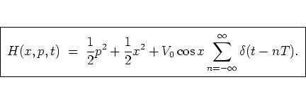 |
(1.9) |
For simplicity, the function
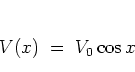 |
(1.10) |
is often referred to as the
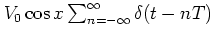
kick potential.1.1It is one of the advantages of the scaling used here that the two
remaining parameters of the system,
the (scaled) period of the perturbation and its (scaled) amplitude
,
concern
only
the kick part of the Hamiltonian.
The unperturbed part of
after scaling
is just a harmonic oscillator with -- formally -- unit
mass and unit frequency.
Note that, while
equation (1.12)
reduces to the Hamiltonian of the CHIRIKOV-TAYLOR map
[Chi79] in the limit  ,
no analogous statement holds for the scaled version
(1.17), since
,
no analogous statement holds for the scaled version
(1.17), since
 is a necessary condition for the
scaling (1.15).
The CHIRIKOV-TAYLOR map is an important standard example of classical
kicked dynamical systems. I return to this map in
subsection 5.1.1, where its bifurcation scenario and
diffusive dynamics are described.
is a necessary condition for the
scaling (1.15).
The CHIRIKOV-TAYLOR map is an important standard example of classical
kicked dynamical systems. I return to this map in
subsection 5.1.1, where its bifurcation scenario and
diffusive dynamics are described.
Footnotes
- ... potential.1.1
-
The
full driving
term
 in equation (1.17) is correctly referred to as a
potential
only
after scaling, i.e. using dimensionless time, as in the present case.
Before scaling, this term has the dimension of energy over time, rather
than energy.
in equation (1.17) is correctly referred to as a
potential
only
after scaling, i.e. using dimensionless time, as in the present case.
Before scaling, this term has the dimension of energy over time, rather
than energy.
Next: Discrete Dynamics
Up: The Kicked Harmonic Oscillator
Previous: Newtonian Equations of Motion
Contents
Martin Engel 2004-01-01