Next: On the Required Number
Up: Singular System Analysis
Previous: Singular Value Decomposition as
Contents
By ``first embedding dimension'' we mean here  , the dimension of the
space with which we begin the procedure described in the last section. We
did not specify yet, but simply said that it should be greater than or
equal to
, the dimension of the
space with which we begin the procedure described in the last section. We
did not specify yet, but simply said that it should be greater than or
equal to  , in order to guarantee that embedding is possible.
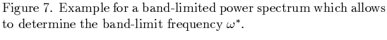
Broomhead and King in [7] suggested to compute the power spectrum,
which shows to which degree the frequencies contribute. Typically, the
power spectrum consists of a noise floor (i.e. all frequencies contribute
equally in the case of white noise) to which the amplitudes due to the
deterministic contribution are added (see Fig. 7).
, in order to guarantee that embedding is possible.
Broomhead and King in [7] suggested to compute the power spectrum,
which shows to which degree the frequencies contribute. Typically, the
power spectrum consists of a noise floor (i.e. all frequencies contribute
equally in the case of white noise) to which the amplitudes due to the
deterministic contribution are added (see Fig. 7).
If the deterministic contribution
is only significant for frequencies which are smaller than some
``band-limit'' frequency  (which corresponds to the
time-interval
(which corresponds to the
time-interval
 )
then one can choose
)
then one can choose  . This can be
justified as follows: On the one hand one wants to make
. This can be
justified as follows: On the one hand one wants to make  large, in order to have it
 (see section 3.1),
on the other hand choosing so large that
(see section 3.1),
on the other hand choosing so large that
 seems not to be sensible, since it is obviously easier
to work with a lower-dimensional embedding space. So the only consistent
a priori estimate seems to be .
Although this justification for the choice of is rather handwaving
and only valid for band-limited data, numerical experiments in
[7] show that in many cases it gives good results.
One reason for this is that most dynamical systems which have been
investigated until now usually have rather low-dimensional attractors
due to the dissipative properties of the systems. This can be true even if
the system is moving in a phase space as high-dimensional as in the case
of the Belousov-Zhabotinski reaction (see chapter 1.1 in [14]).
According to Broomhead and King the choice of the sampling time can
be based on physical considerations as well. Many systems have a
characteristic time-scale: The observables of the system do not change
significantly in times smaller than this. If one decreases
seems not to be sensible, since it is obviously easier
to work with a lower-dimensional embedding space. So the only consistent
a priori estimate seems to be .
Although this justification for the choice of is rather handwaving
and only valid for band-limited data, numerical experiments in
[7] show that in many cases it gives good results.
One reason for this is that most dynamical systems which have been
investigated until now usually have rather low-dimensional attractors
due to the dissipative properties of the systems. This can be true even if
the system is moving in a phase space as high-dimensional as in the case
of the Belousov-Zhabotinski reaction (see chapter 1.1 in [14]).
According to Broomhead and King the choice of the sampling time can
be based on physical considerations as well. Many systems have a
characteristic time-scale: The observables of the system do not change
significantly in times smaller than this. If one decreases  while
keeping the ``window length'' constant then one gets vectors with
more and more components and thus more and more singular values
while
keeping the ``window length'' constant then one gets vectors with
more and more components and thus more and more singular values  .
Doing this one will reach a point where the number
.
Doing this one will reach a point where the number  of those singular
values which are not noise-dominated does not go up further: decreasing
then results essentially in increasing the number of singular
values in the noise floor. This means
that the corresponding value of is small enough to match the
characteristic time of the system and we can take as the sampling
time.
A similar approach to the choice of sampling time is
described by Schuster (chapter 5.3 in [14]): He considers some
fixed and determines as the decay time of the autocorrelation
function
of those singular
values which are not noise-dominated does not go up further: decreasing
then results essentially in increasing the number of singular
values in the noise floor. This means
that the corresponding value of is small enough to match the
characteristic time of the system and we can take as the sampling
time.
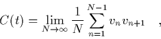
A similar approach to the choice of sampling time is
described by Schuster (chapter 5.3 in [14]): He considers some
fixed and determines as the decay time of the autocorrelation
function  of the time series which can be computed as follows:
 |
(47) |
where  is the time between two successive measurements of
  . Then we
get from
. Then we
get from
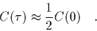 |
(48) |
Since the power spectrum is proportional to the Fourier transform of
the autocorrelation function15 both approaches ([7] and
[14], chapter 5.3) should give comparable estimates for .
Footnotes
- ... function15
-
This is the Wiener-Khinchine theorem.
Next: On the Required Number
Up: Singular System Analysis
Previous: Singular Value Decomposition as
Contents
Martin_Engel
2000-05-25