Next: An Algorithm based on
Up: Analysis of Real-World Data
Previous: Basic Remarks about the
Contents
Schuster [15] proposed to base the choice of  and
and  on
the idea that an embedding using delay coordinates is a topological
mapping which preserves neighbourhood relations. This means that points on
the attractor in
on
the idea that an embedding using delay coordinates is a topological
mapping which preserves neighbourhood relations. This means that points on
the attractor in  which are near to each other should also be near in
the embedding space
which are near to each other should also be near in
the embedding space  .
The distance of any two points
.
The distance of any two points
 cannot decrease
but only increase when one increases the
embedding dimension . But if this distance increases under a change
from to
cannot decrease
but only increase when one increases the
embedding dimension . But if this distance increases under a change
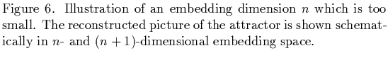
from to  then it is clear that is not sufficiently large,
as Fig. 6 shows.
then it is clear that is not sufficiently large,
as Fig. 6 shows.
being too small means that the attractor is projected onto a space
of lower dimensionality and this projection possibly destroys
neighbourhood relations, resulting in some points appearing nearer to each
other in the embedding space than they actually are.
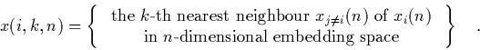
(For example,  may be the nearest neighbour of
  in
although this is not true in the proper embedding space
in
although this is not true in the proper embedding space
 . See, again, Fig. 6 for an illustration of
this observation.) If, on the other hand,
is sufficiently large then the distance of any two points of the
attractor in embedding space should stay the same when one changes
into .
Applying this geometrical point of view, one can find the proper embedding
dimension by
choosing initially a small value of and then increasing it
systematically. One knows that the proper value of is found when all
distances between any two points and do not grow any more
when increasing .
Practically, one constructs the quantity
. See, again, Fig. 6 for an illustration of
this observation.) If, on the other hand,
is sufficiently large then the distance of any two points of the
attractor in embedding space should stay the same when one changes
into .
Applying this geometrical point of view, one can find the proper embedding
dimension by
choosing initially a small value of and then increasing it
systematically. One knows that the proper value of is found when all
distances between any two points and do not grow any more
when increasing .
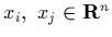
Practically, one constructs the quantity
 |
(22) |
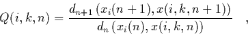
where  is the
  -th reconstructed vector in -dimensional
embedding space,
-th reconstructed vector in -dimensional
embedding space,
 , and
, and
 |
(23) |
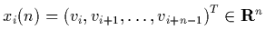
 measures the increase of the distance between and its
 -th nearest neighbour, as increases. (
 is some
appropriate, fixed metric in
.) According to the observations stated above
is some
appropriate, fixed metric in
.) According to the observations stated above  should be
greater than or equal to one. To get a notion what happens not only to the
single point and its neighbours but to all the the next step
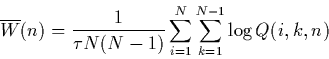
is to calculate
should be
greater than or equal to one. To get a notion what happens not only to the
single point and its neighbours but to all the the next step
is to calculate
 |
(24) |
which considers all  reconstructed points in the embedding space and
all the
reconstructed points in the embedding space and
all the  ``neighbours'' of these10 and adds up the logarithms of the ratios of the respective distances. (The
number of
the increases linearly with , such that there would be a
trivial linear -dependence in
``neighbours'' of these10 and adds up the logarithms of the ratios of the respective distances. (The
number of
the increases linearly with , such that there would be a
trivial linear -dependence in
 . This is removed by
dividing by .)
Clearly, for
equal to the proper embedding dimension and for the right sampling
time ,
should approach zero (within the
experimental
and numerical errors). Thus systematic variation of and seems
to enable us to find sensible values for these quantities. In fact,
numerical experiments done by Schuster [15] show that one can
get reasonable results when using this method.
. This is removed by
dividing by .)
Clearly, for
equal to the proper embedding dimension and for the right sampling
time ,
should approach zero (within the
experimental
and numerical errors). Thus systematic variation of and seems
to enable us to find sensible values for these quantities. In fact,
numerical experiments done by Schuster [15] show that one can
get reasonable results when using this method.
Footnotes
- ... these10
-
To save computing time it is also possible to consider not all the
neighbours of each but only the
 nearest ones.
Next: An Algorithm based on
Up: Analysis of Real-World Data
Previous: Basic Remarks about the
Contents
Martin_Engel
2000-05-25