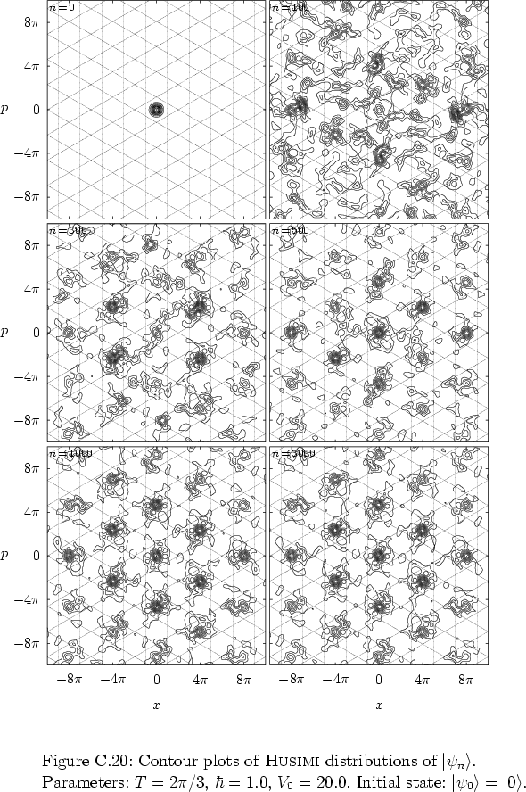
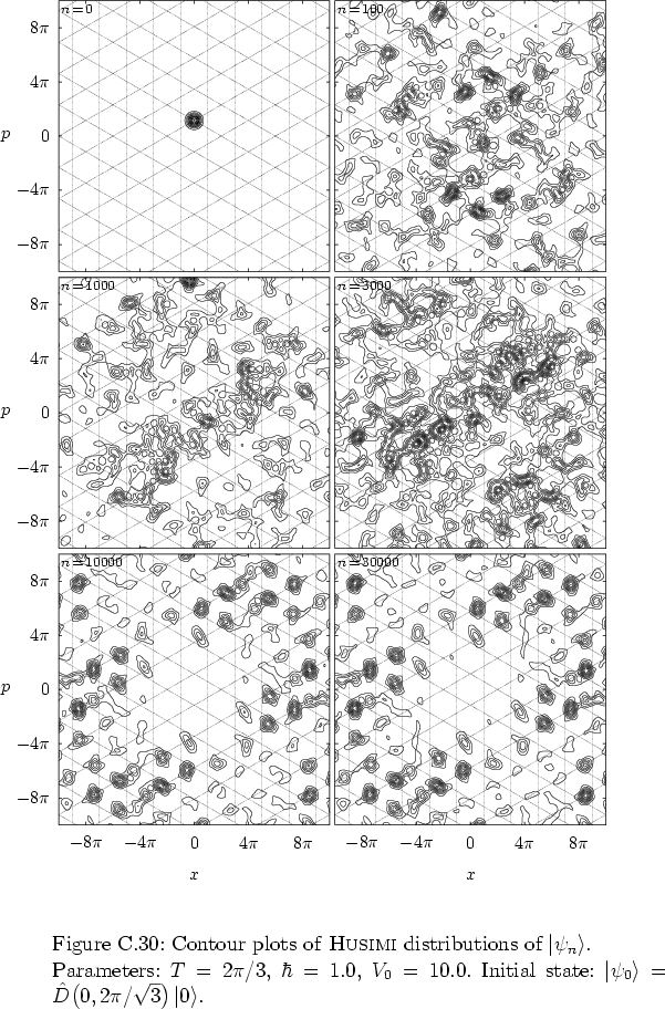
For larger ![]() , the figures
C.20 and
C.31,
using the same parameter values but
, the figures
C.20 and
C.31,
using the same parameter values but ![]() for the former and
for the former and
![]() for the later,
exhibit very similar phase portraits, despite the different initial
conditions.
For
for the later,
exhibit very similar phase portraits, despite the different initial
conditions.
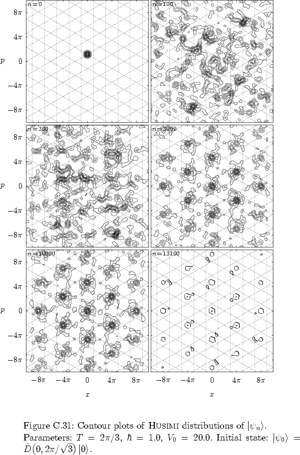
For ![]() ,
figure C.31
shows a (numerical) state the norm of which has already
decayed considerably
(to less than
,
figure C.31
shows a (numerical) state the norm of which has already
decayed considerably
(to less than ![]() ).
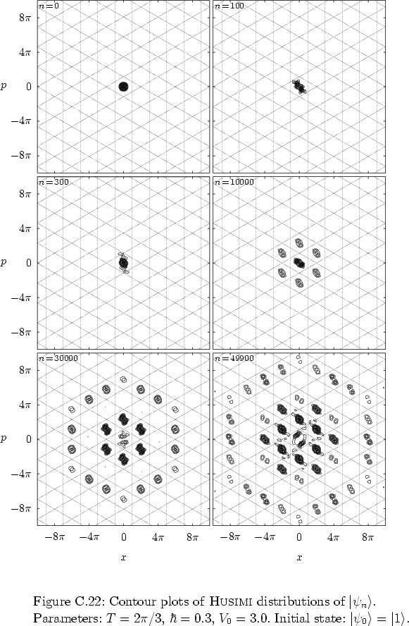
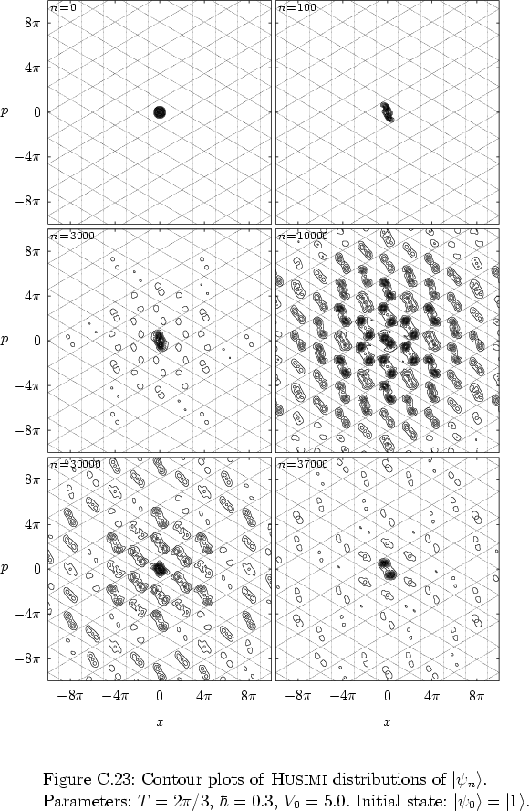
Nevertheless, the most prominent feature of the phase portrait, its
hexagonal structure, is still clearly visible.
).
Nevertheless, the most prominent feature of the phase portrait, its
hexagonal structure, is still clearly visible.
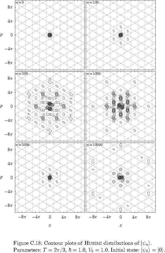
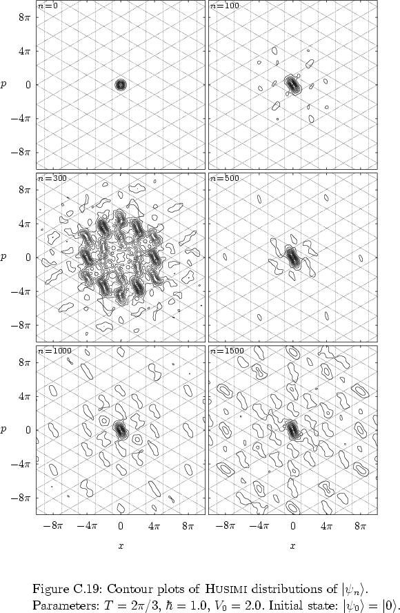
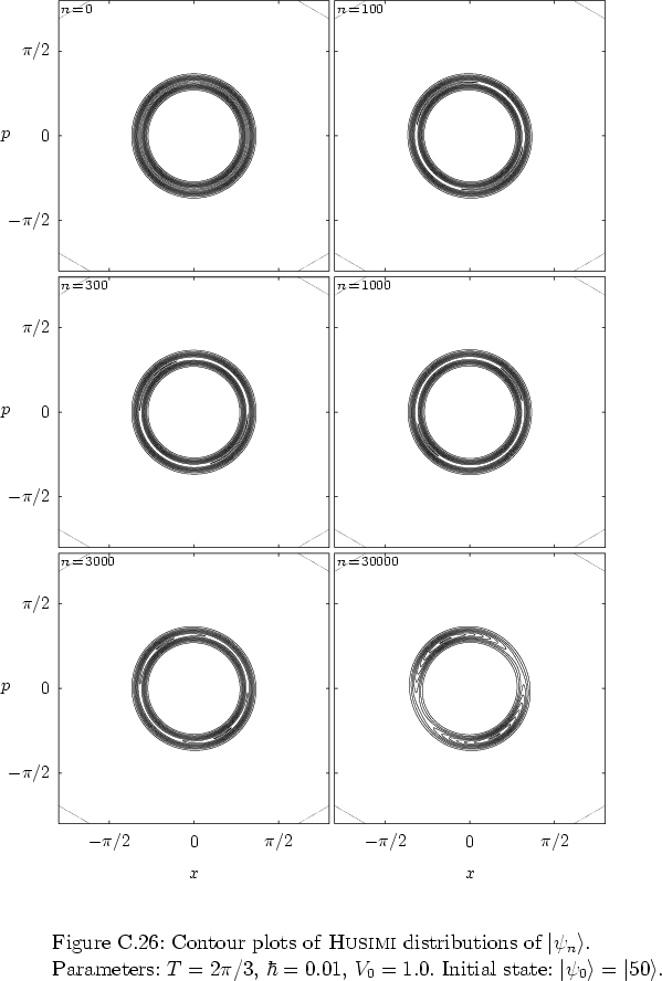
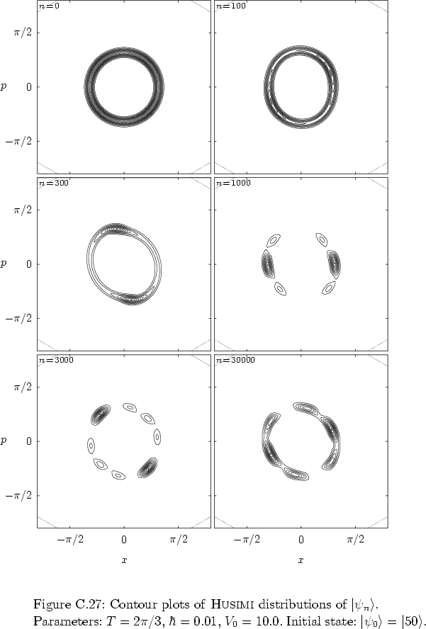
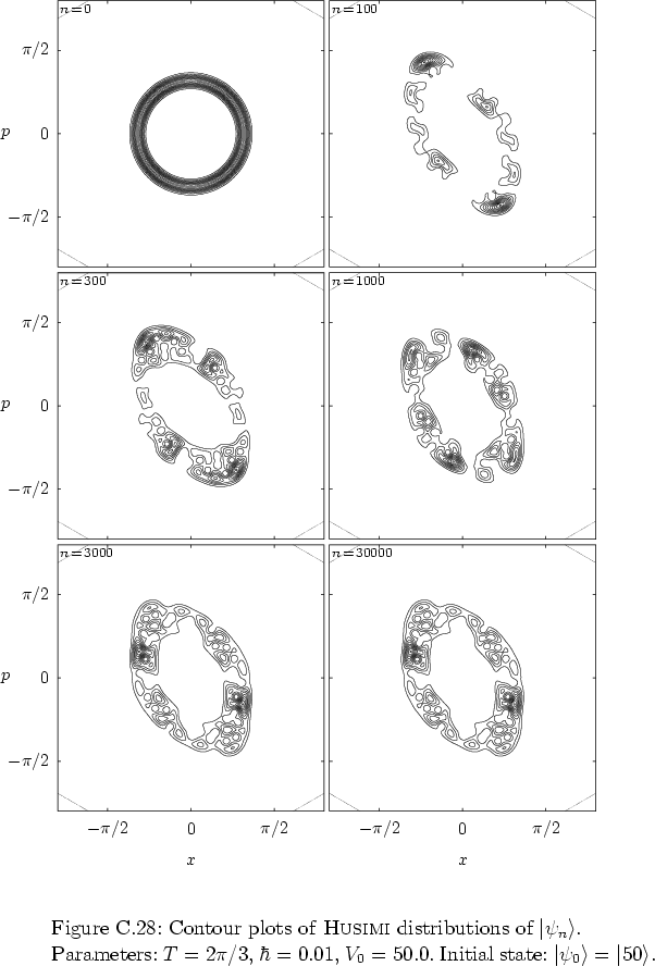
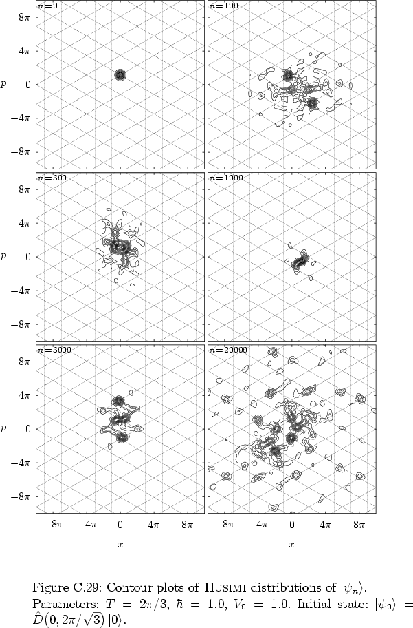
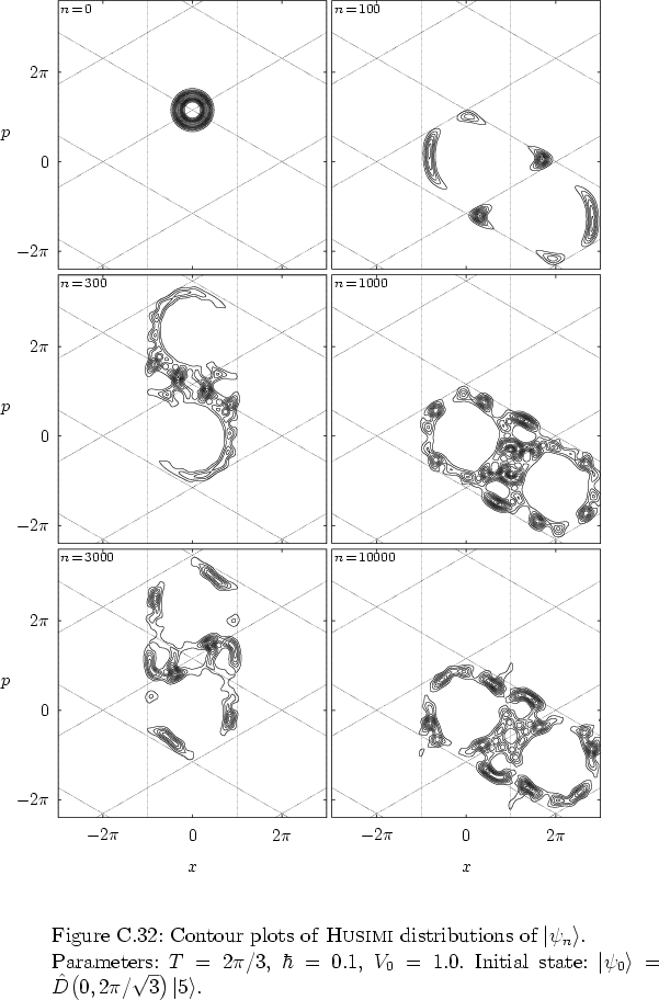
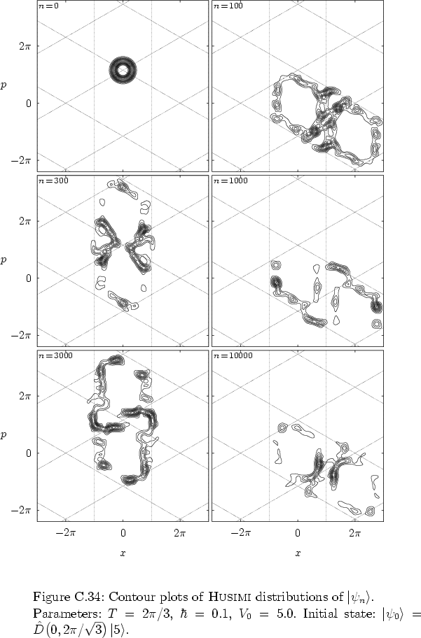
The sequence of figures in the present subsection also nicely demonstrates
some aspects of
the transition from genuinely quantum behaviour (for larger values of
![]() ) to more classical behaviour (for smaller
) to more classical behaviour (for smaller ![]() ):
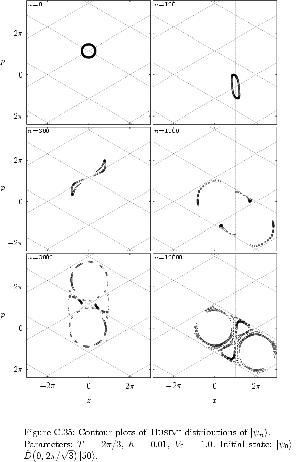
compare
figure C.32
with
figure C.35
and
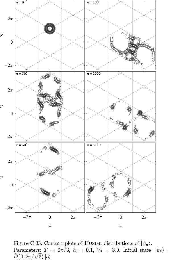
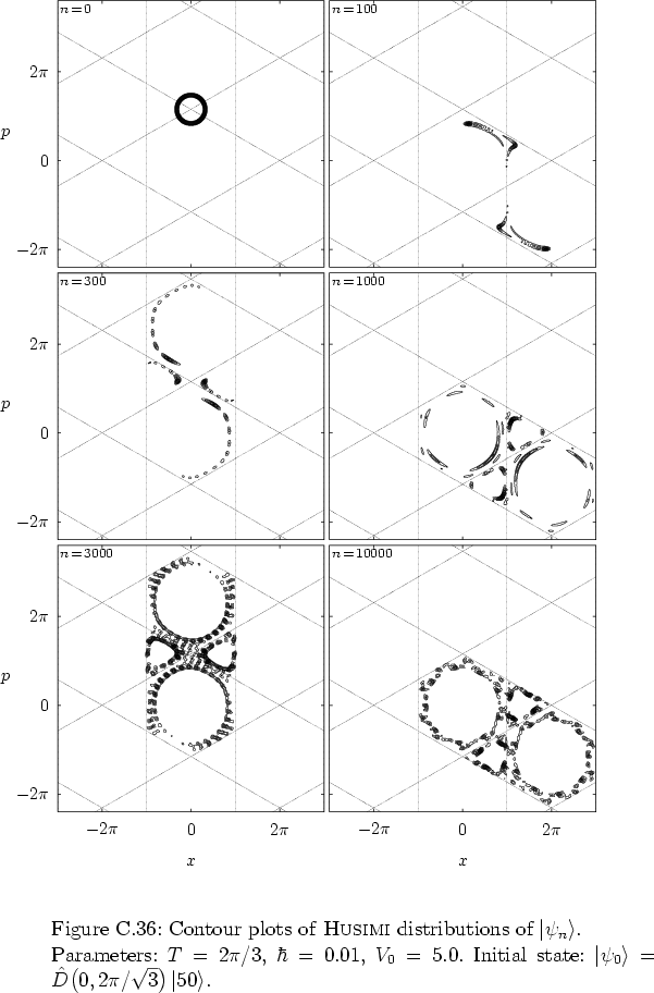
figure C.34
with
figure C.36,
for example.
The smaller value of
):
compare
figure C.32
with
figure C.35
and
figure C.34
with
figure C.36,
for example.
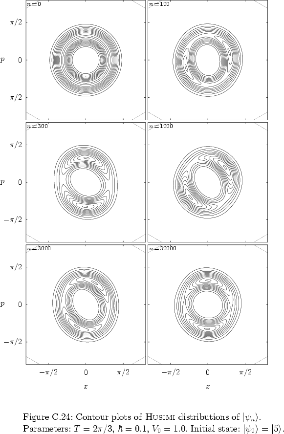
The smaller value of ![]() leads to smaller structures in
phase space, and to a closer resemblance with the classical hexagonal
stochastic web as displayed in figure 1.3a.
leads to smaller structures in
phase space, and to a closer resemblance with the classical hexagonal
stochastic web as displayed in figure 1.3a.
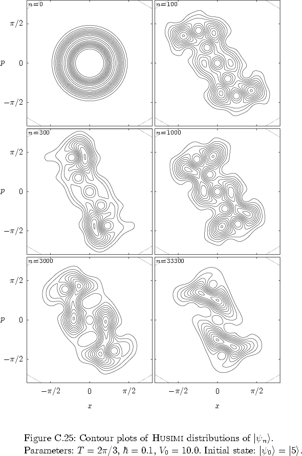
What is more, the figures exhibit some fingerprints
of the classical
POINCARÉ map (1.21) in the quantum phase space dynamics
generated by the quantum map (2.37).
In particular the figures
C.35
(![]() ) and
C.36
(
) and
C.36
(![]() )
apparently
demonstrate the way in which the classical
heteroclinic connections
of the periodic points forming the skeleton of
the web
act as separatrices, separating an incident (part of the)
quantum
wave packet
into two parts that are driven away from the corresponding fixed point
along the unstable manifold of that fixed point.
)
apparently
demonstrate the way in which the classical
heteroclinic connections
of the periodic points forming the skeleton of
the web
act as separatrices, separating an incident (part of the)
quantum
wave packet
into two parts that are driven away from the corresponding fixed point
along the unstable manifold of that fixed point.
The same observations, but for ![]() rather than
rather than ![]() , can
be made with respect to figures
C.12-C.17
and 4.3.
Especially the
figures
4.3 (
, can
be made with respect to figures
C.12-C.17
and 4.3.
Especially the
figures
4.3 (![]() )
and
C.12 (
)
and
C.12 (![]() )
show the
effect
quite clearly. See also
figure 4.5
(
)
show the
effect
quite clearly. See also
figure 4.5
(![]() )
for the same pattern in the quantum
)
for the same pattern in the quantum ![]() -dynamics.
-dynamics.
It should be kept in mind, though,
that these are just phenomenological observations;
the transition from quantum to classical behaviour cannot be described
in these terms in a mathematically sound way. This is reflected by the
fact that for smaller ![]() a (possibly much) larger basis is needed to
describe quantum states in the same region of phase space --
cf. table C.1.
a (possibly much) larger basis is needed to
describe quantum states in the same region of phase space --
cf. table C.1.